---
title: 'Josh''s Notes: 最优阵列处理(Part 1.3 —— 均匀加权线阵)'
mathjax: true
comments: true
copyright: true
toc:
enable: true
number: true
wrap: true
expand_all: true
max_depth: 4
tags:
- 阵列信号处理
- 均匀加权线阵
- 3dB 带宽
- 第一零点波束宽度
- 旁瓣
- 栅瓣
- 瑞利限
categories:
- - Josh 的学习笔记
- 最优阵列处理
- 阵列和空域滤波器
abbrlink: aa32ec76
date: 2023-04-20 19:34:47
---
# 均匀加权线阵的频率-波数响应函数
现在把注意力集中到均匀加权线阵(Uniformly Weighted Linear Array)的情况,即
$$\begin{equation}
w_n = \frac{1}{N}, \, n = 0,1,\cdots,N-1
\end{equation}$$
$$\begin{equation}
\boldsymbol{w} = \frac{1}{N} \boldsymbol{1}
\end{equation}$$
其中 $\boldsymbol{1}$ 是 $N \times 1$ 维的单位矢量,则在 $\psi$ 空间的频率-波数响应函数可以写成(利用等比级数的求和公式)
$$\begin{equation}
\begin{aligned}
\boldsymbol{\varUpsilon}_\psi(\psi) &= \frac{1}{N} \sum_{n=0}^{N-1} e^{j \left(n - \frac{N-1}{2}\right)\psi} \\
&= \frac{1}{N} e^{-j \left(\frac{N-1}{2}\right)\psi} \sum_{n=0}^{N-1} e^{j n \psi} \\
&= \frac{1}{N} e^{-j \left(\frac{N-1}{2}\right)\psi} \left[ \frac{1-e^{jN\psi}}{1-e^{j\psi}} \right]
\end{aligned}
\end{equation}$$
或(利用欧拉公式)
$$\begin{equation}
\boldsymbol{\varUpsilon}_\psi(\psi) = \frac{1}{N} \frac{\sin\left( N \frac{\psi}{2} \right)}{\sin\frac{\psi}{2}}
\end{equation}$$
可以观察到:
- 当 $N$ 是奇数时,$\boldsymbol{\varUpsilon}_\psi(\psi)$ 是周期函数,周期为 $2\pi$;
- 当 $N$ 为偶数时,波瓣在 $\pm 2 \pi$、$\pm 6 \pi$ 处的值为负值,周期为 $4 \pi$;
- 对任意的 $N$,$\left|\boldsymbol{\varUpsilon}_\psi(\psi)\right|$ 的周期为 $2 \pi$。
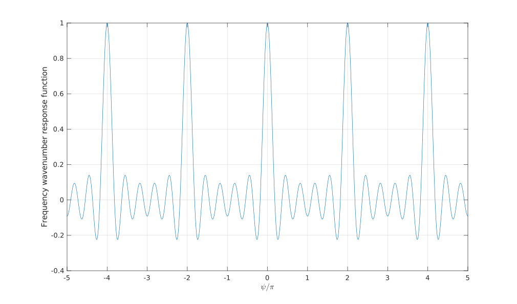
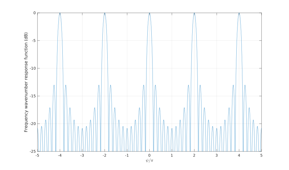
当 $N = 11$ 时, $\boldsymbol{\varUpsilon}_\psi(\psi)$ 和 $\psi$ 的关系在[图 1-3-1](#fig.1-3-1) 中给出。[图 1-3-2](#fig.1-3-2) 给出了 $\left|\boldsymbol{\varUpsilon}_\psi(\psi)\right|$,单位为 dB,其中
$$\begin{equation}
\boldsymbol{\varUpsilon}_\mathrm{dB}(\psi) = 10 \log_{10} \left|\boldsymbol{\varUpsilon}(\psi)\right|^2
\end{equation}$$
{width=1000px}
{width=1000px}
{% note primary MATLAB Code %}
``` matlab fig2_1516.m
%%%%%%%%%%%%%%%%%%%%%%%%%%%%%%%%
% Figure 2.15 & 2.16
% Beampattern of uniformly weighted linear array
% Xiaomin Lu
% Updated 1/5/99
% Last updated by K. Bell 7/22/01, 10/4/01
%%%%%%%%%%%%%%%%%%%%%%%%%%%%%%%%
clear all
close all
N = 11; % 11 elements
% Note, Eq. (2.92) is in fact the standard Dirichlet function
% beam = diric(psi, N);
% if you don't have the signal processing toolbox, this does the same thing
psi = (-5:1/400:5)*pi;
beam = zeros(1,length(psi(:)));
y=sin(.5*psi);
i=find(abs(y)>1e-12); % set where x is not divisible by 2 pi
j=1:length(psi(:));
j(i)=[]; % complement set
beam(i)=sin((N/2)*psi(i))./(N*y(i));
beam(j)=sign(cos(psi(j)*((N+1)/2)));
plot(psi/pi, beam)
grid
xlabel('$\psi/\pi$','Interpreter','latex')
ylabel('Frequency wavenumber response function')
axis([-5 5 -0.4 1])
set(gcf,'Position',[0 0 1000 600])
figure
beam = 20*log10(abs(beam));
plot(psi/pi,beam);
xlabel('$\psi/\pi$','Interpreter','latex')
ylabel('Frequency wavenumber response function (dB)')
axis([-5 5 -25 0])
grid
set(gcf,'Position',[0 0 1000 600])
```
{% endnote %}
若不指定 $\boldsymbol{w}$ 的类型,则 $\boldsymbol{\varUpsilon}_\psi(\psi)$ 是复数,所以相位也应该画出来。但是,均匀加权线阵具有对称性,因此得到的频率-波数响应是实函数。
也可以用 $k_z$ 来表示频率-波数响应
$$\begin{equation}
\boldsymbol{\varUpsilon}(\omega:k_z) = \frac{1}{N} \frac{\sin\left( N k_z \frac{d}{2} \right)}{\sin \left(k_z\frac{d}{2}\right)}
\end{equation}$$
这里 $\boldsymbol{\varUpsilon}(\omega:k_z)$ 是周期函数,周期为 $2\pi/d$。
{% note warning %}
注意,响应函数仅依赖于波数分量 $k_z$,是 $k_z$ 的周期函数,间隔为 $2\pi/d$,这是线性阵列的一维特性导致的,所以该阵列仅能分析在 $k_z$ 方向上投影的波数分量。
{% endnote %}
# 均匀加权线阵的波束方向图
均匀加权线阵的波束方向图为
$$\begin{equation}
B_\theta(\theta) = \frac{1}{N} \frac{\sin\left(\frac{N}{2} \cdot \frac{2\pi}{\lambda} \cos \theta \cdot d \right)}{\sin \left( \frac{1}{2} \cdot \frac{2\pi}{\lambda} \cos\theta \cdot d\right)}, \quad 0 \leqslant \theta \leqslant \pi \\
\end{equation}$$
$$\begin{equation}
B_u(u) = \frac{1}{N} \frac{\sin\left(\frac{ \pi Nd}{\lambda} u \right)}{\sin \left( \frac{N d}{\lambda} u\right)}, \quad -1 \leqslant u \leqslant 1 \label{BeamPatternOfUWLAInDirectionCosineDomain}
\end{equation}$$
$$\begin{equation}
B_\psi(\psi) = \frac{1}{N} \frac{\sin\left(N\frac{\psi}{2}\right)}{\sin \left( \frac{\psi}{2} \right)}, \quad -\frac{2\pi d}{\lambda} \leqslant \psi \leqslant \frac{2\pi d}{\lambda} \label{BeamPatternOfUWLAInWaveNumberDomain}
\end{equation}$$
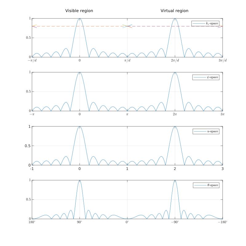
其中定义域分别为 $0 \leqslant \theta \leqslant \pi$、$-1 \leqslant u \leqslant 1$ 和 $-\displaystyle\frac{2\pi d}{\lambda} \leqslant \psi \leqslant \frac{2\pi d}{\lambda}$,称为**{% label primary @可视区域(visible region) %}**。
{% note info %}
函数 $B_u(u)$ 和 $B_\psi(\psi)$ 有时称为**{% label primary @阵列因子(Array Factor) %}**。这个量对非全向性阵元非常重要。
{% endnote %}
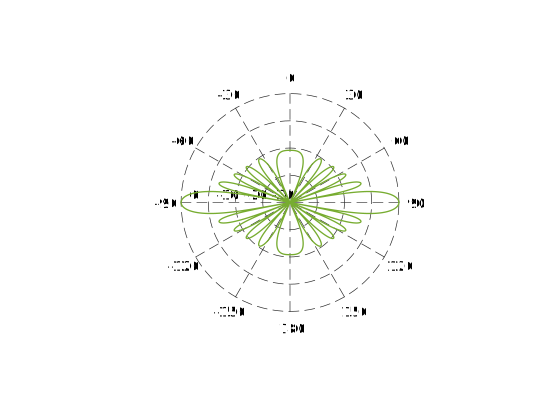
[图 1-3-3](#fig.1-3-3) 给出了 $B_\theta(\theta)$ 的极坐标形式,单位为 dB。如果在三维空间画出波束方向图,在[图 1-3-3](#fig.1-3-3) 中的图将对应沿着任意方位角 $\theta$ 切割得到的方向图。[图 1-3-4](#fig.1-3-4) 给出了波束方向图的幅度和不同变量之间的关系。
{width=800px}
{% note primary MATLAB Code %}
``` matlab fig2_17.m
%%%%%%%%%%%%%%%%%%%%%%%%%%%%%%%%
% Figure 2.17
% Polar plot of B (Theta)
% Lillian Xu 1/5/99
% Updated by K. Bell 6/25/01
% Functions called: polardb
%%%%%%%%%%%%%%%%%%%%%%%%%%%%%%%%
clear all
close all
N = 11; % Elements in array
d = 0.5; % spacing wrt wavelength
beamwidth = 2/(N*d); % null-to-null (LL BW is half this)
D=d*(-(N-1)/2:1:(N-1)/2); % element locations
ang = pi*(-1:0.001:1);
u = cos(ang);
n2=size(u,2);
AS = exp(-1i*2*pi*cos(90/180*pi)*D'); % BP points to 90 (broadside)
Au = exp(-1i*2*pi*D'*u);
B = real(AS'*Au)/N;
G = 20*log10((abs(B)));
h=polardb(ang,G,-40);
```
{% endnote %}
{width=1000px}
{% note primary MATLAB Code %}
``` matlab fig2_18.m
%%%%%%%%%%%%%%%%%%%%%%%%%%%%%%%%
% Figure 2.18
% beam patterns in different spaces
% Lillian Xiaolan Xu
% Last updated 09/07/2000
% updated by K. Bell 7/22/01, 10/4/01
%%%%%%%%%%%%%%%%%%%%%%%%%%%%%%%%
clear all
close all
N = 10;
n = (-(N-1)/2:(N-1)/2).';
psi = pi*(-3:0.001:3);
w = 1/N*[ones(N,1)];
d = 1/2;
vv = exp(1i*2*d*n*psi);
B = (abs(w'*vv));
u1=-1;
u2=3;
y1=0;
y2=1;
subplot(4,1,1)
plot(-psi/d,B);
hold on
axis([u1*pi/d u2*pi/d y1 y2])
set(gca,'XTick',[-pi/d 0 pi/d 2*pi/d 3*pi/d])
set(gca,'YTick',[0 0.5 1])
set(gca,'XTickLabel',{'$-\pi/d$';'$0$';'$\pi/d$';'$2\pi/d$';'$3\pi/d$'}, ...
'TickLabelInterpreter','latex')
grid on
point=0.8;
point_up=0.84;
point_down=0.76;
plot([-pi/d pi/d],[point point],'--')
plot([-1*pi/d -0.9*pi/d],[point point_up])
plot([-1*pi/d -0.9*pi/d],[point point_down])
plot([0.9*pi/d pi/d],[point_up point])
plot([0.9*pi/d pi/d],[point_down point])
text(-0.3*pi/d,1.2,'Visible region')
plot([pi/d 3*pi/d],[point point],'--')
plot([pi/d 1.1*pi/d],[point point_up])
plot([pi/d 1.1*pi/d],[point point_down])
plot([2.9*pi/d 3*pi/d],[point_up point])
plot([2.9*pi/d 3*pi/d],[point_down point])
text(1.7*pi/d,1.2,'Virtual region')
legend({'$k_z$-space'},'Interpreter','latex')
subplot(4,1,2)
plot(psi,B);
hold on
axis([u1*pi u2*pi y1 y2])
set(gca,'XTick',[-pi 0 pi 2*pi 3*pi])
set(gca,'YTick',[0 0.5 1])
set(gca,'XTickLabel',{'$-\pi$';'$0$';'$\pi$';'$2\pi$';'$3\pi$'}, ...
'TickLabelInterpreter','latex')
grid on
legend({'$\psi$-space'},'Interpreter','latex')
subplot(4,1,3)
plot(psi/pi,B);
hold on
axis([u1 u2 y1 y2])
set(gca,'XTick',[-1 0 1 2 3])
set(gca,'YTick',[0 0.5 1])
grid on
legend({'$u$-space'},'Interpreter','latex')
theta = -180:0.1:360;
vv = exp(1i*2*d*n*pi*cos(theta/180*pi));
B = (abs(w'*vv));
subplot(4,1,4)
plot(theta,B);
hold on
axis([-180 180 y1 y2])
set(gca,'XTick',[-180 -90 0 90 180])
set(gca,'YTick',[0 0.5 1])
set(gca,'XTickLabel',{'$180^\circ$';'$90^\circ$';'$0^\circ$';'$-90^\circ$'; ...
'$-180^\circ$'},'TickLabelInterpreter','latex')
grid on
legend({'$\theta$-space'},'Interpreter','latex')
set(gcf,'Position',[0 0 800 800])
```
{% endnote %}
{% note info %}
虽然以上例子比较简单,但是可以用来展示线性阵列的一些重要特征。
{% endnote %}
# 波束方向图的参数
波束方向图的重要特征可以使用波束方向图的参数来描述。
1. 3dB 带宽(半功率波束宽度,half-power beamwidth,HPBW)
2. 到第一零点的距离(这个距离的两倍称为 $BW_{NN}$)
3. 到第一旁瓣的距离
4. 第一旁瓣的高度
5. 其余零点的位置
6. 旁瓣衰减的速率
7. 栅瓣(Grating lobes)
## 半功率波束宽度
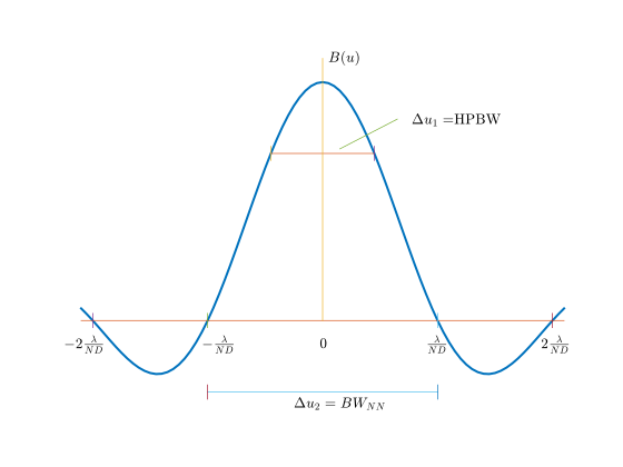
为了说明前两个参数,考虑在[图 1-3-5](#fig.1-3-5) 中给出的原点附近的波束方向图。
{width=700px}
{% note primary MATLAB Code %}
``` matlab fig2_19.m
%%%%%%%%%%%%%%%%%%%%%%%%%%%%%%%%
% Figure 2.19
% Main lobe of beam pattern
% Kristine Bell
% Last updated 6/4/01, 10/4/01
%%%%%%%%%%%%%%%%%%%%%%%%%%%%%%%%
% bp_sect - plots conventional bp with sector
clear all
% close all
%%%%%%%%%%%%%%%%%%%%%%%%%%%%
% Uniform Linear Array
%%%%%%%%%%%%%%%%%%%%%%%%%%%%
N = 10; % Elements in array
d = 0.5; % spacing wrt wavelength
beamwidth = 2/(N*d); % null-to-null (LL BW is half this)
D=d*(-(N-1)/2:1:(N-1)/2); % element locations
u = -0.45:0.01:0.45;
AS = exp(-1i*2*pi*D'*0); % BP points to 0
Au = exp(-1i*2*pi*D'*u);
B = real(AS'*Au)/N; % BP
h=plot(u,B,'-');
set(h,'LineWidth',1.5)
hold on
% HPBW
I=find(B>=0.707);
plot([u(min(I)-1) u(max(I)+1)],[B(min(I)-1) B(max(I)+1)],'-')
plot(u(min(I)-1)*[1 1],B(min(I)-1)*[1 1]+0.03*[-1 1],'-')
plot(u(max(I)+1)*[1 1],B(max(I)+1)*[1 1]+0.03*[-1 1],'-')
plot([0.03 0.13],[0.72 0.845],'-')
text(0.155,0.84,'$\Delta u_1 = $HPBW','Interpreter','latex');
% BW-NN
plot([-0.2 0.2],[-0.3 -0.3],'-')
plot(-0.2*[1 1],-0.3*[1 1]+0.03*[-1 1],'-')
plot(0.2*[1 1],-0.3*[1 1]+0.03*[-1 1],'-')
text(-0.05,-0.35,'$\Delta u_2 = BW_{NN}$','Interpreter','latex');
% axes
plot([-1 1 ],[0 0],'-')
plot([0 0],[-0 1.1],'-')
% tick marks
plot(-0.4*[1 1],0.03*[-1 1])
plot(-0.2*[1 1],0.03*[-1 1])
plot(0.2*[1 1],0.03*[-1 1])
plot(0.4*[1 1],0.03*[-1 1])
yy = -0.1;
%tick labels
text(-0.45,yy,'$-2\frac{\lambda}{ND}$','Interpreter','latex');
text(-0.21,yy,'$-\frac{\lambda}{ND}$','Interpreter','latex');
text(-0.005,yy,'0','Interpreter','latex');
text(0.18,yy,'$\frac{\lambda}{ND}$','Interpreter','latex');
text(0.38,yy,'$2\frac{\lambda}{ND}$','Interpreter','latex');
text(0.01,1.1,'$B(u)$','Interpreter','latex')
hold off
axis([-0.42 0.42 -0.4 1.2])
set(gca,'Visible','off')
```
{% endnote %}
3dB 波束宽度是波束宽度的一个度量。定义为对应 $\left| B_u(u) \right|^2 = 0.5$ 或 $\left| B_u(u) \right| = 1/\sqrt{2}$ 的点。可以通过令波束方向图 $B_u(u)$(式 $\eqref{BeamPatternOfUWLAInDirectionCosineDomain}$)等于 $1/\sqrt{2}$,来求出 $u$ 空间的半功率点。对于 $N\geqslant 10$,通过解下面的方程可以得到一个很好的近似:
$$\begin{equation}
\frac{\pi N d}{\lambda} u = 1.4
\end{equation}$$
即有
$$\begin{equation} \label{ApproximationOfHPBW}
\Delta u_1 = 0.891 \frac{\lambda}{N d}
\end{equation}$$
我们把这个间隔称为**{% label primary @半功率波束宽度(half-power beamwidth,HPBW) %}**。当 $N$ 增加时,式 $\eqref{ApproximationOfHPBW}$ 中的常系数会稍稍减小。对于 $N > 30$,$0.886 \lambda/Nd$ 是一个更好的近似表达式。
[表 1-3-1](#table.1-3-1) 中列出了不同空间内 HPBW 的表达式。
表 1-3-1 各个空间的半功率波束宽度
|空间| 任意 $d$ | $d=\lambda/2$ |
| :--: | :------: | :------: |
| $u$ | $0.891 \frac{\lambda}{Nd}$ | $1.782 \frac{1}{N}$ |
| $\bar{\theta}$ [^1] | $2\sin^{-1} \left( 0.446 \frac{\lambda}{Nd} \right)$ | $2\sin^{-1} \left( 0.891 \frac{1}{N} \right)$ |
| 较小的 $\bar{\theta}$ | $\simeq 0.891 \frac{\lambda}{Nd}$ radians
$\simeq 51.05 \frac{\lambda}{Nd}$ degrees | $\simeq 1.782 \frac{1}{N}$ radians
$\simeq 102.1 \frac{1}{N}$ degrees |
| $\psi$ | $0.891 \frac{2\pi}{N}$ | $0.891 \frac{2\pi}{N}$ |
| $k_z$ | $0.891 \frac{2\pi}{dN}$ | $1.782 \frac{2\pi}{\lambda N}$ |
[^1]: 侧射角(broadside angle)的定义为 $\bar{\theta} = \pi/2 - \theta$
## 第一零点波束宽度
方向图的零点出现在当波束方向图 $B_u(u)$(式 $\eqref{BeamPatternOfUWLAInDirectionCosineDomain}$)的分子为零而分母不为零时,即
$$\begin{equation}
\sin \left( \frac{\pi N d}{\lambda} u \right) = 0
\end{equation}$$
成立的条件为
$$\begin{equation}
\frac{\pi N d}{\lambda} u = m\pi, \quad m = 1,2,\cdots
\end{equation}$$
则出现零点需要满足下面的两个条件:
$$\begin{equation}
u = m \frac{\lambda}{Nd}, \quad m = 1,2,\cdots
\end{equation}$$
且
$$\begin{equation}
u \ne m \frac{\lambda}{d}, \quad m = 1,2,\cdots
\end{equation}$$
则第一个零点的位置为 $\lambda/Nd$,即有
$$\begin{equation}
\Delta u_2 = 2 \frac{\lambda}{Nd}
\end{equation}$$
我们把 $\Delta u_2$ 称为零点-零点波束宽度(null-to-null beamwidth),用 $BW_{NN}$ 表示。 $BW_{NN}$ 的一半是到第一零点的距离 ($0.5 BW_{NN}$) 。这个量能够衡量阵列分辨两个不同平面波的能力,也称为{% label primary @瑞利限(Rayleigh resolution limit) %}。如果第二个波束方向图的峰值在第一个波束方向图的第一零点之外(间隔 $\geqslant \Delta u_2 / 2$),则认为这两个平面波是可以分辨的。在后面,我们将研究一个阵列的分辨能力的统计性度量。
{% note warning %}
注意到线阵在方位角方向($\varphi$)没有分辨能力,因为该阵列在 $x$ 和 $y$ 方向上没有扩展。我们将在后面详细讨论分辨率的问题。
{% endnote %}
[表 1-3-2](#table.1-3-2)中列出了在各个不同空间表示出的 $BW_{NN}$。
表 1-3-2 各个空间的第一零点波束宽度
|空间| 任意 $d$ | $d=\lambda/2$ |
| :--: | :------: | :------: |
| $u$ | $2 \frac{\lambda}{Nd}$ | $\frac{4}{N}$ |
| $\bar{\theta}$ | $2\sin^{-1} \left( \frac{\lambda}{Nd} \right)$ | $2\sin^{-1} \left( \frac{2}{N} \right)$ |
| 较小的 $\bar{\theta}$ | $\simeq 2 \frac{\lambda}{Nd}$ radians | $\simeq \frac{4}{N}$ radians |
| $\psi$ | $\frac{4\pi}{N}$ | $\frac{4\pi}{N}$ |
| $k_z$ | $\frac{4\pi}{dN}$ | $\frac{8\pi}{\lambda N}$ |
## 旁瓣的位置及其衰减速率
旁瓣极大值的位置出现在当波束方向图 $B_\psi(\psi)$(式 $\eqref{BeamPatternOfUWLAInWaveNumberDomain}$)中的分子逼近极大值的时候:
$$\begin{equation}
\sin \left( \frac{N \psi}{2} \right) = 1
\end{equation}$$
则此时有
$$\begin{equation}
\frac{N \psi}{2} = \pm \left( 2m+1 \right)\frac{\pi}{2}, \quad m = 1,2,\cdots
\end{equation}$$
也即在 $\psi$ 空间有
$$\begin{equation}
\psi = \pm \frac{2m+1}{N}\pi
\end{equation}$$
也即在 $u$ 空间有
$$\begin{equation}
u = \pm \frac{2m+1}{N}\frac{\lambda}{2d}
\end{equation}$$
则第一旁瓣的峰值出现在
$$\begin{equation}
\psi = \pm \frac{2\pi}{N}
\end{equation}$$
由于在极大值时,波束方向图 $B_\psi(\psi)$(式 $\eqref{BeamPatternOfUWLAInWaveNumberDomain}$)中的分子趋近为 1,因此极大值为
$$\begin{equation}
B_\psi \left( \pm \frac{3\pi}{N} \right) \approx \frac{1}{N \sin \left( \frac{3\pi}{2N} \right)}
\end{equation}$$
对于较大的 $N$,这个表达式可以进一步近似为
$$\begin{equation}
B_\psi \left( \pm \frac{3\pi}{N} \right) \approx \frac{3}{2\pi}
\end{equation}$$
计算得 -13.5dB。
{% note warning %}
这意味着一个信号如果在这个旁瓣的位置入射,且比位置在 $k_z = 0$ 的信号大 13.5dB,则这两个信号将产生相同的响应。主要的旁瓣出现在 $k_z = \pm(2m + 1) \pi/Nd$,旁瓣的水平衰减速率为 $1/(2m + 1)$。例如,第二旁瓣的高度为 -17.9dB。在实际中,这种旁瓣水平的分辨能力是不能被接受的,所以很少使用均匀加权。旁瓣控制在确定性阵列和自适应阵列设计中都是特别重要的问题。
{% endnote %}
## 栅瓣(Grating lobes)
{width=1000px}
{% note primary MATLAB Code %}
``` matlab fig2_20.m
%%%%%%%%%%%%%%%%%%%%%%%%%%%%%%%%
% Figure 2.20
% Effect of element spacing on beam pattern
% Xin Zhang
% Lillian Xu updated 09/2000
% updated by K. Bell 7/22/2001, 10/4/01
%%%%%%%%%%%%%%%%%%%%%%%%%%%%%%%%
clear all
close all
N = 10;
n = (-(N-1)/2:(N-1)/2).';
psi = pi*(-3:0.001:3);
w = 1/N*[ones(N,1)];
d = [1/4 1/2 1];
figure
for k =1:length(d)
vv = exp(1i*2*d(k)*n*psi);
B(k,:) = 20*log10(abs(w'*vv));
subplot(3,1,k)
plot(psi/pi,B(k,:));
hold on
plot([-1 -1],[-25 0],'--');
plot([1 1],[-25 0],'--');
axis([-3 3 -25 5])
set(gca,'YTick',[-25 -20 -15 -10 -5 0])
grid on
xlabel('$u$','Interpreter','latex')
if k == 1
plot([-1 1],[2.5 2.5])
plot([-1 -0.9],[2.5 0.5])
plot([-1 -0.9],[2.5 4.5])
plot([0.9 1],[0.5 2.5])
plot([0.9 1],[4.5 2.5])
text(-0.4,7,'Visible region')
end
hold off
end
set(gcf,'Position',[0 0 800 600])
```
{% endnote %}
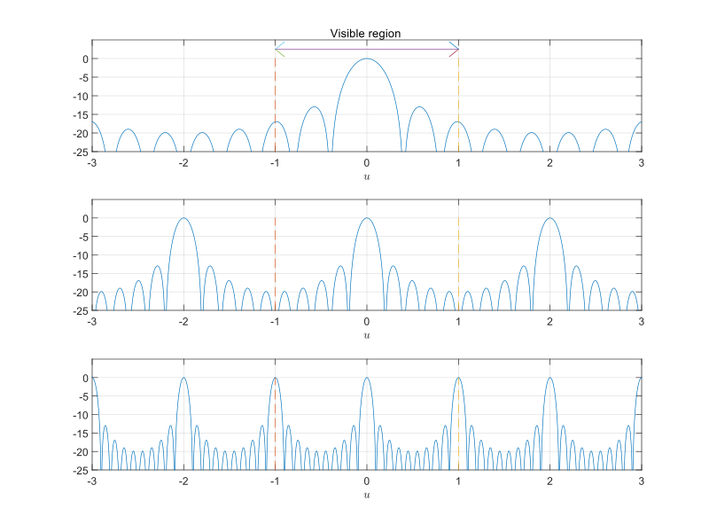
在[图 1-3-6](#fig.1-3-6) 中,针对多种 $d/\lambda$ 的值,画出了 $\left| \boldsymbol{\varUpsilon}_u(u) \right|$。图中说明了“栅瓣”这个重要的概念,即和主波束一样高的波瓣。栅瓣发生在当波束方向图 $B_\psi(\psi)$(式 $\eqref{BeamPatternOfUWLAInWaveNumberDomain}$)中的分子和分母均为零的时候。栅瓣出现的间隔为
$$\begin{equation}
\frac{\psi}{2} = m \cdot \pi
\end{equation}$$
也即
$$\begin{equation}
\psi = m \cdot 2 \pi
\end{equation}$$
也即
$$\begin{equation}
u = m \cdot \frac{\lambda}{d}
\end{equation}$$
如果阵列的间距大于 $\lambda$,则栅瓣的峰值出现在信号传播区域以内,即在 $\left| u \right| \leqslant 1$ 的区域以内。这里就会出现峰值响应模糊的问题,只有当我们对信号的入射方向有先验信息的时候,才可能解决这个问题。
下一节将讨论阵列调向的问题,阵列调向使得在 $u$ 空间的频率-波数响应函数 $\left| \boldsymbol{\varUpsilon}_u(u) \right|$ 发生平移,这种平移导致栅瓣进入了可视区域以内。我们发现,如果阵列需要的调向范围为 $0^\circ \leqslant \theta \leqslant 180^\circ$ 则需要
$$\begin{equation}
\frac{d}{\lambda} \leqslant \frac{1}{2}
\end{equation}$$
也即
$$\begin{equation}
\lambda \leqslant \frac{\lambda}{2}
\end{equation}$$
通常,我们考虑满足 $d \leqslant \lambda/2$ 的阵列,并假设需要在整个球内进行调向。我们把满足 $d = \lambda/2$ 的均匀线阵称为**{% label primary @标准线阵(standard linear array) %}**。
{% note info %}
在时间序列分析中,当对时域波形欠采样时,会出现混迭问题。栅瓣的问题和时域混迭问题是等同的。
{% endnote %}
# 参考文献
1. Van Trees, Harry L. *Optimum array processing: Part IV of detection, estimation, and modulation theory.* John Wiley & Sons, 2002.
2. Van Trees, Harry L, 汤俊. *最优阵列处理技术.* 清华大学出版社. 2008.