
125 lines
5.3 KiB
Markdown
125 lines
5.3 KiB
Markdown
---
|
||
title: 'Josh''s Notes: 最优阵列处理(Part 1.1 —— 频率-波数响应和波束方向图)'
|
||
mathjax: true
|
||
comments: true
|
||
copyright: true
|
||
toc:
|
||
enable: false
|
||
number: true
|
||
wrap: true
|
||
expand_all: true
|
||
max_depth: 4
|
||
categories:
|
||
- - Josh 的学习笔记
|
||
- 最优阵列处理
|
||
- 阵列和空域滤波器
|
||
abbrlink: 8b61f5a7
|
||
date: 2023-04-18 23:57:47
|
||
tags:
|
||
- 阵列信号处理
|
||
- 频率-波数响应
|
||
- 波束方向图
|
||
---
|
||
|
||
  假设在空时场的某个区域内有一个或多个信号,同时在某些区域内存在噪声和/或干扰。在一些阵列信号处理的应用场景中,这些区域是部分重叠的。阵列可以利用信号的空域特征,对空时场域(space-time field)内的信号进行滤波。这种滤波可以用一种与角度或波数的相关性(in terms of a dependence upon angle or wavenumber)进行描述。在频域看,这种滤波是通过使用复增益对阵列输出进行加权,根据信号的空域相关性对信号进行增强或抑制来实现的。通常我们对空时场进行空域滤波的目的是:使得从一个(或一组)特定角度到来的信号通过有效的组合得到增强,抑制从其他角度到来的噪声或干扰。
|
||
|
||
<a id="fig.1-1-1"></a>
|
||
|
||
{width=600px}
|
||
|
||
  首先需要明确采用的坐标系,如[图 1-1-1](#fig.1-1-1) 所示,直角坐标系和球坐标系的关系也在其中标明:
|
||
|
||
$$\begin{equation}
|
||
\begin{aligned}
|
||
x &= r \sin\theta\cos\varphi \\
|
||
y &= r \sin\theta\sin\varphi \\
|
||
z &= r \cos\theta
|
||
\end{aligned}
|
||
\end{equation}$$
|
||
|
||
<!-- more -->
|
||
|
||
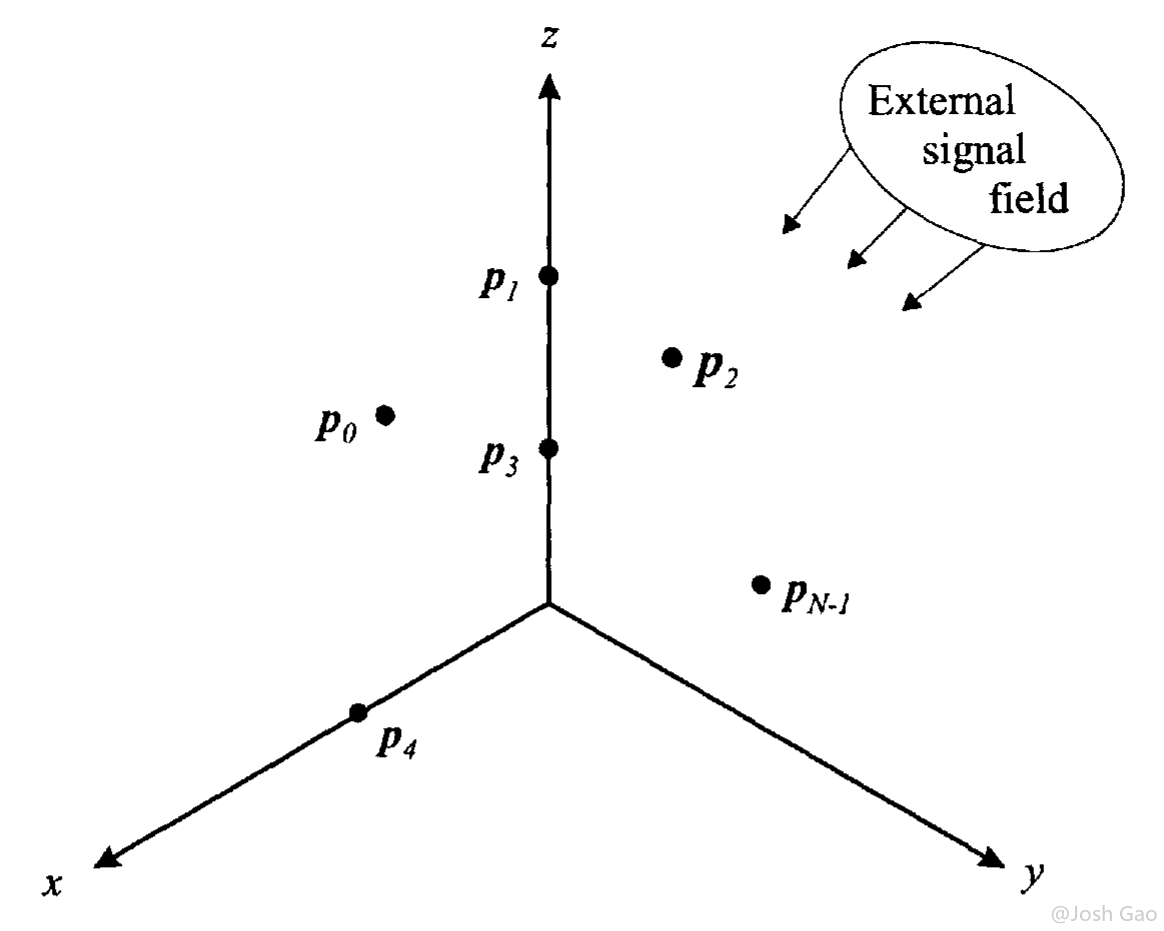
  本文分析一个阵列对外部信号场的响应。阵列由一组全向阵元组成,阵元的位置为 $\vec{p}_n$,如[图 1-1-2](#fig.1-1-2) 所示。阵元在位置 $\vec{p}_n : n = 0, 1, \cdots, N — 1$ 上对信号场进行空域采样。这产生了一组信号,表示为矢量 $\vec{f}\left(t, \vec{p}\right)$
|
||
|
||
$$\begin{equation}
|
||
\vec{f}(t, \vec{p}) = \left[
|
||
\begin{array}{c}
|
||
f\left(t, \vec{p}_0\right) \\
|
||
f\left(t, \vec{p}_1\right) \\
|
||
\vdots \\
|
||
f\left(t, \vec{p}_{N-1}\right) \\
|
||
\end{array}
|
||
\right]
|
||
\end{equation}$$
|
||
|
||
<a id="fig.1-1-2"></a>
|
||
|
||
{width=600px}
|
||
|
||
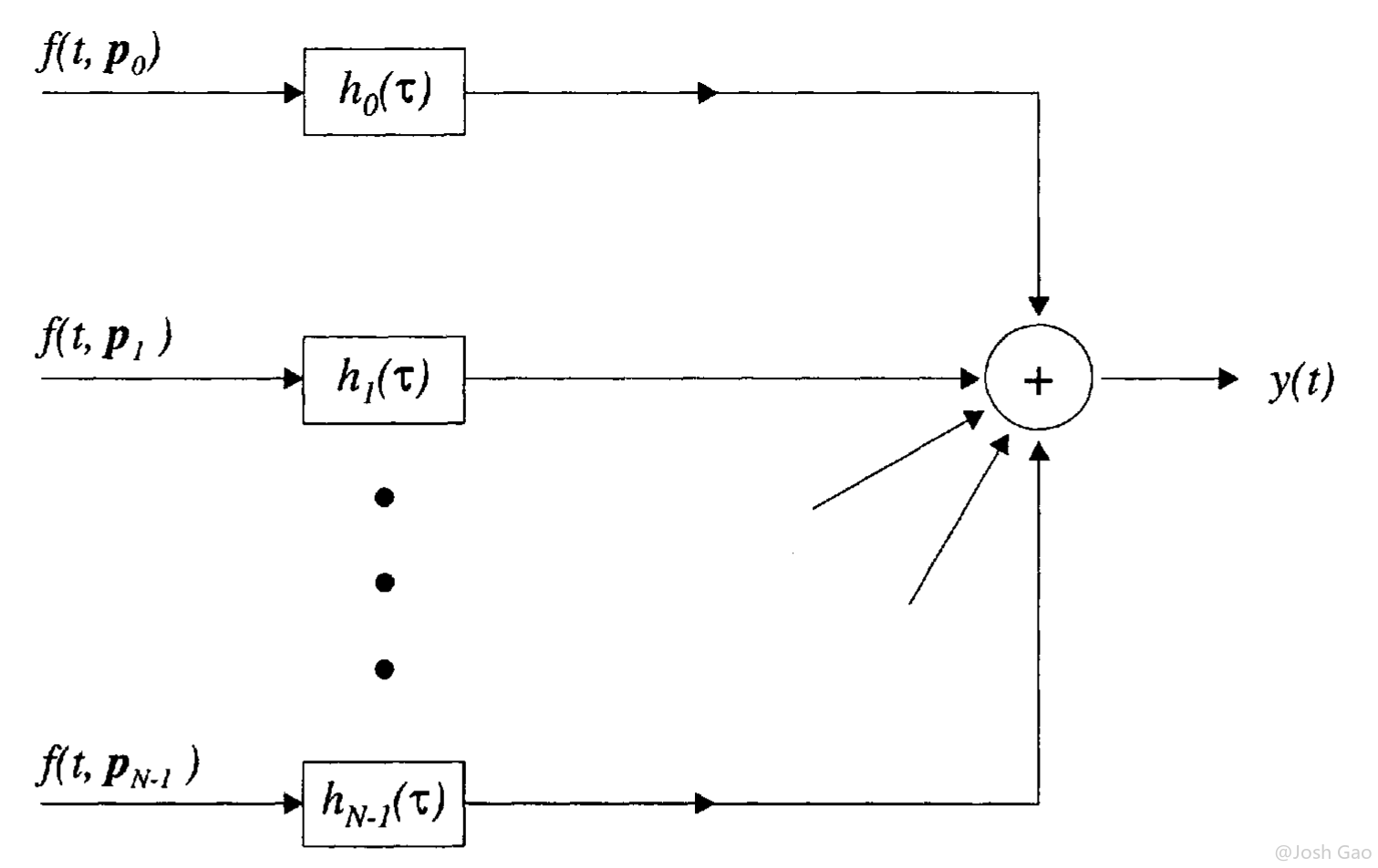
  对每个阵元的输出用一个线性时不变滤波器进行处理,该滤波器的冲激响应为 $h_n(\tau)$
|
||
并对所有输出求和,得到阵列的输出 $y(t)$,如[图 1-1-3](#fig.1-1-3) 所示。假设观察间隔足够长(可以考虑为无限长),则输出 $y(t)$ 可以写成一个卷积积分的形式:
|
||
|
||
$$\begin{equation}
|
||
y(t) = \sum_{n=0}^{N-1} \int_{-\infty}^{\infty} h_n (t-\tau)f_n\left(\tau,\vec{p}_n\right) \mathrm{d} \tau
|
||
\end{equation}$$
|
||
|
||
<a id="fig.1-1-3"></a>
|
||
|
||
{width=600px}
|
||
|
||
这个结果可以用矢量符号表示为(即将标量结果向矢量模型的进行直接扩展,a straightforward extension of scalar results to the vector model)
|
||
|
||
$$\begin{equation} \label{VectorFormOfLinearArrayOutputInTimeDomain}
|
||
y(t) = \int_{-\infty}^{\infty} \vec{h}^\mathrm{T} (t-\tau) \vec{f}\left(\tau,\vec{p}\right) \mathrm{d} \tau
|
||
\end{equation}$$
|
||
|
||
其中
|
||
|
||
$$\begin{equation}
|
||
\vec{h}(\tau) = \left[ \begin{array}{c}
|
||
h_0(\tau) \\
|
||
h_1(\tau) \\
|
||
\vdots \\
|
||
h_{N-1}(\tau)
|
||
\end{array}
|
||
\right]
|
||
\end{equation}$$
|
||
|
||
也可以把式 $\eqref{VectorFormOfLinearArrayOutputInTimeDomain}$ 在变换域表示为
|
||
|
||
$$\begin{equation}
|
||
\begin{aligned}
|
||
Y(\omega) &= \int_{-\infty}^{\infty} y(t) e^{-j\omega t} \mathrm{d} t \\
|
||
&= \vec{H}^\mathrm{T}(\omega) \vec{F}(\omega)
|
||
\end{aligned}
|
||
\end{equation}$$
|
||
|
||
其中
|
||
|
||
$$\begin{equation}
|
||
\vec{H} (\omega) = \int_{-\infty}^{\infty} \vec{h}(t) e^{-j\omega t} \mathrm{d} t
|
||
\end{equation}$$
|
||
|
||
$$\begin{equation} \label{SampleVectorInFreqDomain}
|
||
\vec{F} \left(\omega,\vec{p}\right) = \int_{-\infty}^{\infty} \vec{f}\left(\tau,\vec{p}\right) e^{-j\omega t} \mathrm{d} t
|
||
\end{equation}$$
|
||
|
||
在大多数情况下,去掉 $\eqref{SampleVectorInFreqDomain}$ 中左边的 $\vec{p}$, 直接使用 $\vec{F}(\omega)$ 。
|
||
|
||
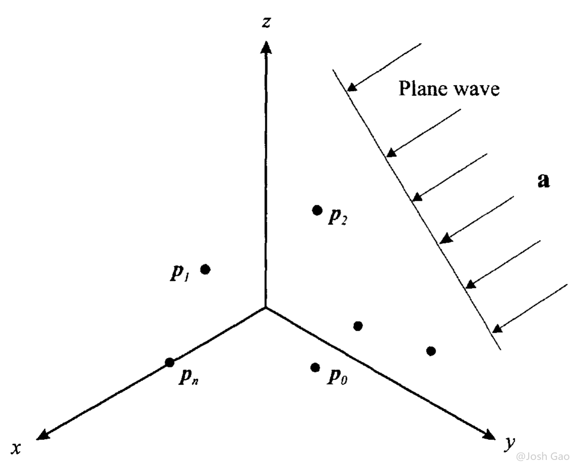
下面考虑[图 1-1-4](#fig.1-1-4) 所示的简单的波束形成的操作。输入是一个平面波,传播方向为 $\vec{a}$, 时域频率(弧度)为 $\omega$。由该输入而产生的传感器的时间函数可以用两种等效的方式进行表示。第一种方式强调由千在不同的传感器上的不同到达时间而对应的时间延时。设 $f(t)$ 是在坐标系原点接收到的信号,则
|
||
|
||
<a id="fig.1-1-4"></a>
|
||
|
||
{width=600px}
|
||
|
||
$$\begin{equation}
|
||
\vec{f}(t, \vec{p}) = \left[
|
||
\begin{array}{c}
|
||
f\left(t - \tao_0\right) \\
|
||
f\left(t - \tao_1\right) \\
|
||
\vdots \\
|
||
f\left(t - \tao_{N-1}\right) \\
|
||
\end{array}
|
||
\right]
|
||
\end{equation}$$
|