update toc structure

some blog contents are alse modified

_config.next.yml

@@ -42,7 +42,7 @@ custom_file_path:
 scheme: Gemini
 
 # Dark Mode
-darkmode: false
+darkmode: true
 
 
 # ---------------------------------------------------------------
@@ -66,8 +66,8 @@ creative_commons:
   license: by-nc-sa
   # Available values: big | small
   size: small
-  sidebar: true
+  sidebar: false
-  post: false
+  post: true
   # You can set a language value if you prefer a translated version of CC license, e.g. deed.zh
   # CC licenses are available in 39 languages, you can find the specific and correct abbreviation you need on https://creativecommons.org
   language: deed.zh
@@ -158,13 +158,13 @@ social:
   E-Mail: mailto:[email protected] || fa fa-envelope
   #Weibo: https://weibo.com/yourname || fab fa-weibo
   #Google: https://plus.google.com/yourname || fab fa-google
-  #Twitter: https://twitter.com/yourname || fab fa-twitter
+  #Twitter: https://twitter.com/josh_gao || fab fa-twitter
   #FB Page: https://www.facebook.com/yourname || fab fa-facebook
   #StackOverflow: https://stackoverflow.com/yourname || fab fa-stack-overflow
   #YouTube: https://youtube.com/yourname || fab fa-youtube
   #Instagram: https://instagram.com/yourname || fab fa-instagram
   #Skype: skype:yourname?call|chat || fab fa-skype
-  CSDN: https://josh-gao.blog.csdn.net/ || fab fa-cuttlefish
+  CSDN: https://blog.csdn.net/weixin_43870101 || fab fa-cuttlefish
 
 social_icons:
   enable: true
@@ -188,11 +188,11 @@ toc:
   # Automatically add list number to toc.
   number: true
   # If true, all words will placed on next lines if header width longer then sidebar width.
-  wrap: true # controlled only by top level
+  wrap: false # controlled only by top level
   # If true, all level of TOC in a post will be displayed, rather than the activated part of it.
   expand_all: false # controlled only by top level
   # Maximum heading depth of generated toc.
-  max_depth: 3
+  max_depth: 4
 
 
 # ---------------------------------------------------------------
@@ -339,7 +339,7 @@ calendar:
 
 # Preload styles and preconnect CDN for fonts and plugins.
 # For more information: https://www.w3.org/TR/resource-hints/#preconnect
-preconnect: false
+preconnect: true
 
 # Set the text alignment in posts / pages.
 text_align:
@@ -386,7 +386,7 @@ back2top:
 
 # Reading progress bar
 reading_progress:
-  enable: false
+  enable: true
   # Available values: left | right
   start_at: left
   # Available values: top | bottom
@@ -397,12 +397,12 @@ reading_progress:
 
 # Bookmark Support
 bookmark:
-  enable: true
+  enable: false
   # Customize the color of the bookmark.
   color: "#222"
   # If auto, save the reading progress when closing the page or clicking the bookmark-icon.
   # If manual, only save it by clicking the bookmark-icon.
-  save: auto
+  save: manual
 
 # `Follow me on GitHub` banner in the top-right corner.
 github_banner:
@@ -490,7 +490,7 @@ yandex_site_verification:
 
 # Baidu Webmaster tools verification.
 # See: https://ziyuan.baidu.com/site
-baidu_site_verification:
+baidu_site_verification: codeva-qqFHulQHkE
 
 
 # ---------------------------------------------------------------
@@ -574,7 +574,7 @@ math:
 
 # Easily enable fast Ajax navigation on your website.
 # For more information: https://github.com/next-theme/pjax
-pjax: false
+pjax: true
 
 # FancyBox is a tool that offers a nice and elegant way to add zooming functionality for images.
 # For more information: https://fancyapps.com/fancybox/
@@ -602,8 +602,8 @@ quicklink:
 
   # Home page and archive page can be controlled through home and archive options below.
   # This configuration item is independent of `enable`.
-  home: false
+  home: true
-  archive: false
+  archive: true
 
   # Default (true) will initialize quicklink after the load event fires.
   delay: true
@@ -700,8 +700,8 @@ disqusjs:
 # For more information: https://changyan.kuaizhan.com
 changyan:
   enable: false
-  appid:
+  appid: cywCjT2Ce
-  appkey:
+  appkey: c413e82874f27a2ebad90047ce54c0c1
   # Show comments count
   count: true
 
@@ -759,14 +759,14 @@ add_this_id:
 # Google Analytics
 # See: https://analytics.google.com
 google_analytics:
-  tracking_id: # <app_id>
+  tracking_id: G-FS8FDJ89QM
   # By default, NexT will load an external gtag.js script on your site.
   # If you only need the pageview feature, set the following option to true to get a better performance.
   only_pageview: false
 
 # Baidu Analytics
 # See: https://tongji.baidu.com
-baidu_analytics: # <app_id>
+baidu_analytics: 350182f3e243a2a441aad7e64040d3ce
 
 # Growingio Analytics
 # See: https://www.growingio.com
@@ -774,7 +774,7 @@ growingio_analytics: # <project_id>
 
 # Cloudflare Web Analytics
 # See: https://www.cloudflare.com/web-analytics/
-cloudflare_analytics:
+cloudflare_analytics: 97f59b7e4ea54bd79d9c911c06f990de
 
 # Microsoft Clarity Analytics
 # See: https://clarity.microsoft.com/

_config.yml

@@ -67,7 +67,7 @@ prismjs:
 # order_by: Posts order. (Order by date descending by default)
 index_generator:
   path: ''
-  per_page: 15
+  per_page: 10
   order_by: -date
 
 # Category & Tag
@@ -90,7 +90,7 @@ updated_option: 'mtime'
 
 # Pagination
 ## Set per_page to 0 to disable pagination
-per_page: 10
+per_page: 15
 pagination_dir: page
 
 # Include / Exclude file(s)
@@ -107,15 +107,18 @@ theme: next
 # Deployment
 ## Docs: https://hexo.io/docs/one-command-deployment
 deploy:
+  - type: git
+    repo: [email protected]:/home/josh/documents/josh-blog-deploy.git
+    branch: master
+  - type: git
+    repo: [email protected]:/home/josh/documents/josh-blog.git
+    branch: master
   - type: git
     repo: [email protected]:josh-gao/josh-blog/josh-blog.git
     branch: master
   - type: git
     repo: [email protected]:JoshGao-bit/JoshGao-bit.github.io.git
     branch: master
-  - type: git
-    repo: [email protected]:/data/josh_blog.git
-    branch: master
 
 # MathJax [Redundant]
 # math:
@@ -193,3 +196,15 @@ neat_js:
     - '**/jquery.fancybox.pack.js'
     - '**/index.js'
     - '**/fireworks.js'
+
+related_posts:
+  enabled: true
+  filter_threshold: 0.13
+  related_count: 3
+  weight:
+    title: 0.1
+    description: 0
+    keywords: 0
+    tags: 0.01
+    categories: 0.05
+    text: 0

package-lock.json

@@ -21,6 +21,7 @@
         "hexo-helper-live2d": "^3.1.1",
         "hexo-neat": "^1.0.9",
         "hexo-related-popular-posts": "^5.0.1",
+        "hexo-related-posts": "^1.5.1",
         "hexo-renderer-ejs": "^2.0.0",
         "hexo-renderer-pandoc": "^0.3.1",
         "hexo-renderer-stylus": "^2.1.0",
@@ -96,6 +97,15 @@
         "node": ">=0.4.0"
       }
     },
+    "node_modules/afinn-165": {
+      "version": "1.0.4",
+      "resolved": "https://registry.npmjs.org/afinn-165/-/afinn-165-1.0.4.tgz",
+      "integrity": "sha512-7+Wlx3BImrK0HiG6y3lU4xX7SpBPSSu8T9iguPMlaueRFxjbYwAQrp9lqZUuFikqKbd/en8lVREILvP2J80uJA==",
+      "funding": {
+        "type": "github",
+        "url": "https://github.com/sponsors/wooorm"
+      }
+    },
     "node_modules/agent-base": {
       "version": "6.0.2",
       "resolved": "https://registry.npmmirror.com/agent-base/-/agent-base-6.0.2.tgz",
@@ -223,6 +233,17 @@
         "node": ">= 8"
       }
     },
+    "node_modules/apparatus": {
+      "version": "0.0.10",
+      "resolved": "https://registry.npmjs.org/apparatus/-/apparatus-0.0.10.tgz",
+      "integrity": "sha512-KLy/ugo33KZA7nugtQ7O0E1c8kQ52N3IvD/XgIh4w/Nr28ypfkwDfA67F1ev4N1m5D+BOk1+b2dEJDfpj/VvZg==",
+      "dependencies": {
+        "sylvester": ">= 0.0.8"
+      },
+      "engines": {
+        "node": ">=0.2.6"
+      }
+    },
     "node_modules/aproba": {
       "version": "1.2.0",
       "resolved": "https://registry.npmmirror.com/aproba/-/aproba-1.2.0.tgz",
@@ -4433,6 +4454,18 @@
         "node": ">=0.10.0"
       }
     },
+    "node_modules/hexo-related-posts": {
+      "version": "1.5.1",
+      "resolved": "https://registry.npmjs.org/hexo-related-posts/-/hexo-related-posts-1.5.1.tgz",
+      "integrity": "sha512-KeNGQXcfsDKGyP66wiUVlcqguMyBn0n9tsFE5CftxhD9jiOrCmsqCibY1Aq8w/9f92+uxl+NlNkFhkrLezRFVg==",
+      "dependencies": {
+        "natural": "^2.1.5"
+      },
+      "peerDependencies": {
+        "chalk": "^4.1.0",
+        "hexo": "^4.2.0 || ^5.2.0 || ^6.3.0"
+      }
+    },
     "node_modules/hexo-renderer-ejs": {
       "version": "2.0.0",
       "resolved": "https://registry.npmmirror.com/hexo-renderer-ejs/-/hexo-renderer-ejs-2.0.0.tgz",
@@ -5909,6 +5942,17 @@
       "resolved": "https://registry.npmmirror.com/json-schema-traverse/-/json-schema-traverse-0.4.1.tgz",
       "integrity": "sha512-xbbCH5dCYU5T8LcEhhuh7HJ88HXuW3qsI3Y0zOZFKfZEHcpWiHU/Jxzk629Brsab/mMiHQti9wMP+845RPe3Vg=="
     },
+    "node_modules/json-stable-stringify": {
+      "version": "1.0.2",
+      "resolved": "https://registry.npmjs.org/json-stable-stringify/-/json-stable-stringify-1.0.2.tgz",
+      "integrity": "sha512-eunSSaEnxV12z+Z73y/j5N37/In40GK4GmsSy+tEHJMxknvqnA7/djeYtAgW0GsWHUfg+847WJjKaEylk2y09g==",
+      "dependencies": {
+        "jsonify": "^0.0.1"
+      },
+      "funding": {
+        "url": "https://github.com/sponsors/ljharb"
+      }
+    },
     "node_modules/json-stringify-safe": {
       "version": "5.0.1",
       "resolved": "https://registry.npmmirror.com/json-stringify-safe/-/json-stringify-safe-5.0.1.tgz",
@@ -5925,6 +5969,14 @@
         "node": ">=6"
       }
     },
+    "node_modules/jsonify": {
+      "version": "0.0.1",
+      "resolved": "https://registry.npmjs.org/jsonify/-/jsonify-0.0.1.tgz",
+      "integrity": "sha512-2/Ki0GcmuqSrgFyelQq9M05y7PS0mEwuIzrf3f1fPqkVDVRvZrPZtVSMHxdgo8Aq0sxAOb/cr2aqqA3LeWHVPg==",
+      "funding": {
+        "url": "https://github.com/sponsors/ljharb"
+      }
+    },
     "node_modules/jsonparse": {
       "version": "1.3.1",
       "resolved": "https://registry.npmmirror.com/jsonparse/-/jsonparse-1.3.1.tgz",
@@ -6782,6 +6834,22 @@
         "node": ">=0.10.0"
       }
     },
+    "node_modules/natural": {
+      "version": "2.4.5",
+      "resolved": "https://registry.npmjs.org/natural/-/natural-2.4.5.tgz",
+      "integrity": "sha512-fxQou4ubo6Rzf7XL0jjwtC2vHm6Sdicu7ztcE0k1ODZs+d1UzcKF1Hu2IwE2y7OgzU3Sa9o8obw7rnyNrjsd1A==",
+      "dependencies": {
+        "afinn-165": "^1.0.2",
+        "apparatus": "^0.0.10",
+        "json-stable-stringify": "^1.0.1",
+        "sylvester": "^0.0.12",
+        "underscore": "^1.9.1",
+        "wordnet-db": "^3.1.11"
+      },
+      "engines": {
+        "node": ">=0.4.10"
+      }
+    },
     "node_modules/ncp": {
       "version": "2.0.0",
       "resolved": "https://registry.npmmirror.com/ncp/-/ncp-2.0.0.tgz",
@@ -9206,6 +9274,14 @@
         "node": ">= 0.4"
       }
     },
+    "node_modules/sylvester": {
+      "version": "0.0.12",
+      "resolved": "https://registry.npmjs.org/sylvester/-/sylvester-0.0.12.tgz",
+      "integrity": "sha512-SzRP5LQ6Ts2G5NyAa/jg16s8e3R7rfdFjizy1zeoecYWw+nGL+YA1xZvW/+iJmidBGSdLkuvdwTYEyJEb+EiUw==",
+      "engines": {
+        "node": ">=0.2.6"
+      }
+    },
     "node_modules/symbol-tree": {
       "version": "3.2.4",
       "resolved": "https://registry.npmmirror.com/symbol-tree/-/symbol-tree-3.2.4.tgz",
@@ -9519,6 +9595,11 @@
         "node": ">=0.8.0"
       }
     },
+    "node_modules/underscore": {
+      "version": "1.13.6",
+      "resolved": "https://registry.npmjs.org/underscore/-/underscore-1.13.6.tgz",
+      "integrity": "sha512-+A5Sja4HP1M08MaXya7p5LvjuM7K6q/2EaC0+iovj/wOcMsTzMvDFbasi/oSapiwOlt252IqsKqPjCl7huKS0A=="
+    },
     "node_modules/union-value": {
       "version": "1.0.1",
       "resolved": "https://registry.npmmirror.com/union-value/-/union-value-1.0.1.tgz",
@@ -9954,6 +10035,14 @@
         "node": ">=0.10.0"
       }
     },
+    "node_modules/wordnet-db": {
+      "version": "3.1.14",
+      "resolved": "https://registry.npmjs.org/wordnet-db/-/wordnet-db-3.1.14.tgz",
+      "integrity": "sha512-zVyFsvE+mq9MCmwXUWHIcpfbrHHClZWZiVOzKSxNJruIcFn2RbY55zkhiAMMxM8zCVSmtNiViq8FsAZSFpMYag==",
+      "engines": {
+        "node": ">=0.6.0"
+      }
+    },
     "node_modules/wrappy": {
       "version": "1.0.2",
       "resolved": "https://registry.npmmirror.com/wrappy/-/wrappy-1.0.2.tgz",

package.json

@@ -25,6 +25,7 @@
     "hexo-helper-live2d": "^3.1.1",
     "hexo-neat": "^1.0.9",
     "hexo-related-popular-posts": "^5.0.1",
+    "hexo-related-posts": "^1.5.1",
     "hexo-renderer-ejs": "^2.0.0",
     "hexo-renderer-pandoc": "^0.3.1",
     "hexo-renderer-stylus": "^2.1.0",

scaffolds/draft.md

@@ -1,4 +1,14 @@
 ---
 title: {{ title }}
 tags:
+categories:
+mathjax: true
+comments: true
+copyright: true
+toc:
+  enable: true
+  number: ture
+  wrap: true
+  expand_all: true
+  max_depth: 4
 ---

scaffolds/post.md

@@ -2,4 +2,14 @@
 title: {{ title }}
 date: {{ date }}
 tags:
+categories:
+mathjax: true
+comments: true
+copyright: true
+toc:
+  enable: true
+  number: ture
+  wrap: true
+  expand_all: true
+  max_depth: 4
 ---

source/_data/styles.styl

@@ -1,298 +1,34 @@
 // Custom styles.
 
-// 网站最顶部条线的颜色
-// .headband {
-//   height: 3px;
-//   background: #222222;
-// }
-
 // 设置背景图片
 body{
-    // background:url('https://josh-blog-1257563604.cos.ap-beijing.myqcloud.com/img/backgroud.jpg');
+  // background:url('https://josh-blog-1257563604.cos.ap-beijing.myqcloud.com/img/backgroud.jpg');
-    background:url(../images/bg.svg);
+  background:url(../images/bg.svg);
-    background-repeat:repeat;
+  background-repeat:repeat;
-    // background-attachment:fixed;
+  // background-attachment:fixed;
-    // background-position:center;
+  // background-position:center;
-    // background-size:100% 100%;
+  // background-size:100% 100%;
 }
 
-// 设置侧边栏左上角网站标题和副标题区颜色
+// 博客内容透明化
-// .site-meta {
+// :root {
-// 	background: #222222;
+//   --content-bg-color:rgba(255, 255, 255, 0.96);
 // }
 
-// 设置侧边栏网站标题样式
+@media (prefers-color-scheme: light) {
-.site-title {
+  :root {
-
+    --content-bg-color:rgba(255, 255, 255, 0.96);
+  }
 }
 
-// 设置侧边栏网站标题鼠标悬浮样式
+@media (prefers-color-scheme: dark) {
-// .site-title:hover {
+  :root {
-// 	letter-spacing: 0.1rem;
+    --content-bg-color:rgba(0, 0, 0, 0.88);
-// }
+  }
-
-// 侧边栏网站副标题样式
-// .site-subtitle {
-// 	color:#fff;
-// }
-
-// 文章标题鼠标悬浮下划线样式
-// .posts-expand .post-title-link::before {
-// 	content: "";
-//     position: absolute;
-//     width: 100%;
-//     height: 2px;
-//     bottom: 0;
-//     left: 0;
-//     background-color: #222222;
-//     visibility: hidden;
-//     transform: scaleX(0);
-//     transition-duration: 0.2s;
-//     transition-timing-function: ease-in-out;
-//     transition-delay: 0s;
-// }
-
-// // 文章标题颜色
-// .posts-expand .post-title-link {
-// 	color:#222222;
-// }
-
-// // 阅读全文按钮样式
-// .btn {
-// 	border:2px solid #222222;
-// 	color:#222222;
-// }
-
-// // 阅读全文按钮鼠标悬浮样式
-// .btn:hover {
-//   border-color: #222222;
-//   color: #fff;
-//   background: #222222;
-// }
-
-// // 设置文章和侧边栏中链接样式
-// a:hover,
-// span.exturl:hover {
-//   color: #222222;
-//   border-bottom-color: #222222;
-// }
-
-// // 修改文章页侧边栏文章目录下面的第一个标题的鼠标悬浮样式
-// // 真的有毒，文章目录第一个标题的样式还是单独设置的...一开始还没发现
-// .post-toc .nav .active-current > a:hover {
-//     color: #222222;
-// }
-
-// // 文章页面左边文章标题颜色
-// .post-toc ol a:hover {
-//   color: #222222;
-//   border-bottom-color: #222222;
-// }
-
-// // 文章页面左边文章标题active时颜色
-// .post-toc .nav .active > a {
-//   color: #222222;
-//   border-bottom-color: #222222;
-// }
-
-// // 文章页侧边栏文章目录和站点概况鼠标悬浮样式
-// .sidebar-nav li:hover {
-//   color: #222222;
-// }
-
-// // 文章页侧边栏文章目录和站点概况active时鼠标悬浮样式
-// .sidebar-nav .sidebar-nav-active:hover {
-//   color: #222222;
-// }
-
-// // 文章页侧边栏文章目录和站点概况active时样式
-// .sidebar-nav .sidebar-nav-active {
-//   color: #222222;
-//   border-bottom-color: #222222;
-// }
-
-// // 社交栏鼠标悬浮样式
-// #sidebar div.links-of-author.motion-element a:hover {
-//   color: #222222;
-//   background: rgba(255, 255, 255, 0);
-// }
-
-// // 友链鼠标悬浮样式
-// .sidebar a:hover,
-// .sidebar span.exturl:hover {
-//   border-bottom-color: #222222;
-//   color: #222222;
-// }
-
-// RSS文字颜色
-//#sidebar div.feed-link.motion-element > a {
-//  color: #222222;
-//}
-
-// RSS图标颜色
-//#sidebar div.feed-link.motion-element > a i{
-//  color: #222222;
-//}
-
-// 侧边栏日志、分类、标签 上面的数字的颜色
-// .site-state-item-count {
-//   color: #222222;
-// }
-
-// 设置底部文章分页数字鼠标悬浮上划线颜色
-// .pagination .prev:hover,
-// .pagination .next:hover,
-// .pagination .page-number:hover {
-//   border-top-color: #222222;
-// }
-
-// 设置文章页上一篇文章和下一篇文章鼠标悬浮样式
-// .post-nav-item a:hover {
-//   color: #222222;
-//   border-bottom: none;
-// }
-
-// 修改鼠标选中字符的颜色
-/* webkit, opera, IE9 */
-// ::selection {
-//     background: #222222;
-//     color: #f7f7f7;
-// }
-/* firefox */
-// ::-moz-selection {
-//     background: #222222;
-//     color: #f7f7f7;
-// }
-
-// 侧边栏返回顶部按钮鼠标悬浮样式
-// .back-to-top:hover {
-//   background: #eee;
-//   color: #222222;
-// }
-
-// 当页面处于 首页、标签、分类、归档、关于页面其中之一时，处于哪个页面哪个选项就变蓝
-// #menu > li.menu-item-active > a {
-//   color: #222222;
-// }
-
-// 侧边栏导航小圆点颜色
-// .menu-item-active a:after,
-// .menu .menu-item a:hover:after,
-// .menu .menu-item span.exturl:hover:after {
-//   background-color: #222222;
-// }
-
-// 侧边栏上半部分设置为透明
-.menu-item-active a,
-.menu .menu-item a:hover,
-.menu .menu-item span.exturl:hover {
-  background: rgba(255, 255, 255, 0);
-  border-bottom-color: rgba(255, 255, 255, 0);;
 }
 
-// 侧边栏下半部分设置为透明
-.sidebar{
-	background: rgba(255, 255, 255, 0);
-}
-.sidebar-inner{
-	background: rgba(255, 255, 255, 0.94);
-}
-
-// 设置底部文章分页部分为透明
-.pagination{
-	background: rgba(255, 255, 255, 0.94);
-}
-.pagination .page-number.current {
-  color: #fff;
-  background: #222222;
-}
-
-// 导航栏底部百分比透明
-.back-to-top,
-.back-to-top:hover
-{
-	background: rgba(255, 255, 255, 0);
-}
-
-// 设置文章背景透明度
-.post-block{
-	background: rgba(255, 255, 255, 0.94);
-}
-
-// 这里需要完全透明，不然就会在上面的0.7基础上再进行透明度计算
-.btn{
-	background: rgba(255, 255, 255, 0);
-}
-
-.header-inner{
-	background: rgba(255, 255, 255, 0.94);
-}
-.main-inner {
-    background: rgba(255, 255, 255, 0.94);
-}
-
-// 代码高亮背景透明
-// .table-container{
-// 	background: rgba(29, 31, 33, 0.94);
-// }
-// table > tbody > tr:nth-of-type(odd) {
-//   background-color: rgba(29, 31, 33, 0);
-// }
-// table > tbody > tr:hover {
-//   background-color: rgba(29, 31, 33, 0);
-// }
-// pre,
-// .highlight {
-//   background: rgba(29, 31, 33, 0);
-// }
-// .highlight .gutter pre {
-//   background: rgba(29, 31, 33, 0.94);
-// }
-// .highlight .code pre {
-//   background: rgba(29, 31, 33, 0);
-// }
-
-// 评论
-.comments {
-  background: rgba(255, 255, 255, 0.94);
-}
-
-// 文章页内作者信息
-.post-copyright {
-  border-left: 3px solid #222222;
-  background: rgba(255, 255, 255, 0.3);
-}
-
-/* 行内代码块的自定义样式 */
-// code {
-//     color: #222222;
-//     background: rgba(220,220,220, 0.94);
-//     margin: 2px;
-//     border: 1px solid #90EE90;
-// }
-
-// 底部动态的叶子图标
-// .with-love{
-// 	color: green;
-// }
-
-// 去掉文章白色背景
-.main-inner {
-  background: rgba(255,255,255,0);
-}
-
-// // 标签页链接下划线颜色
-// a,
-// span.exturl {
-//   border-bottom: 1px solid #222222;
-// }
-
-// // 标签页链接鼠标悬浮颜色
-// .tag-cloud a:hover {
-//   color: #222222 !important;
-// }
-
 
+// 修复不蒜子显示属性被 hexo-helper-live2d 覆盖
 #busuanzi_container_site_uv, #busuanzi_container_site_pv, #busuanzi_container_page_pv {
   display: inline !important;
 }

source/_posts/2020-11-25-matlab-rcosdesign.md

@@ -3,19 +3,18 @@ title: MATLAB 函数 —— rcosdesign
 tags:
   - MATLAB
   - 翻译
-  - 成型滤波器
+  - 成形滤波器
   - 滤波器
 categories:
-  - - MATLAB
+  - [MATLAB, 函数用法]
-  - - 翻译
-    - 帮助文档
 mathjax: true
 copyright: true
+comments: true
 abbrlink: 5c45edfe
 date: 2020-11-25 22:32:42
 ---
 
-`rcosdesign`：升余弦 FIR 脉冲成型滤波器设计
+`rcosdesign`：升余弦 FIR 脉冲成形滤波器设计
 
 # 语法
 
@@ -32,32 +31,30 @@ date: 2020-11-25 22:32:42
 
 # 示例
 
-## 设计根升余弦滤波器<span id="Examples-01"></span>
+## 设计根升余弦滤波器<a name="Examples-01"></a>
 
 将滚降系数设为 `0.25`，波器的符号数设为 `6`，每个符号 `4` 个采样点。验证 `sqrt` 是 `shape` 参数的默认值。
 
-```m
+``` matlab
 h = rcosdesign(0.25,6,4);
 mx = max(abs(h-rcosdesign(0.25,6,4,'sqrt')))
 ```
 
 > <font face="Consolas">mx = 0</font><br>
 
-```m
+``` matlab
 fvtool(h,'Analysis','impulse')
 ```
 
-<div align="center">
+![ ](https://josh-blog-1257563604.cos.ap-beijing.myqcloud.com/img/2020-11-25-matlab-rcosdesign/2020-11-25-matlab-rcosdesign-010-DesignASquareRootRaisedCosineFilterExample-01.png?imageMogr2/thumbnail/!100p|watermark/2/text/QEpvc2ggR2Fv/font/YWhyb25iZC50dGY=/fontsize/14/dissolve/20/gravity/southeast/dx/5/dy/5)
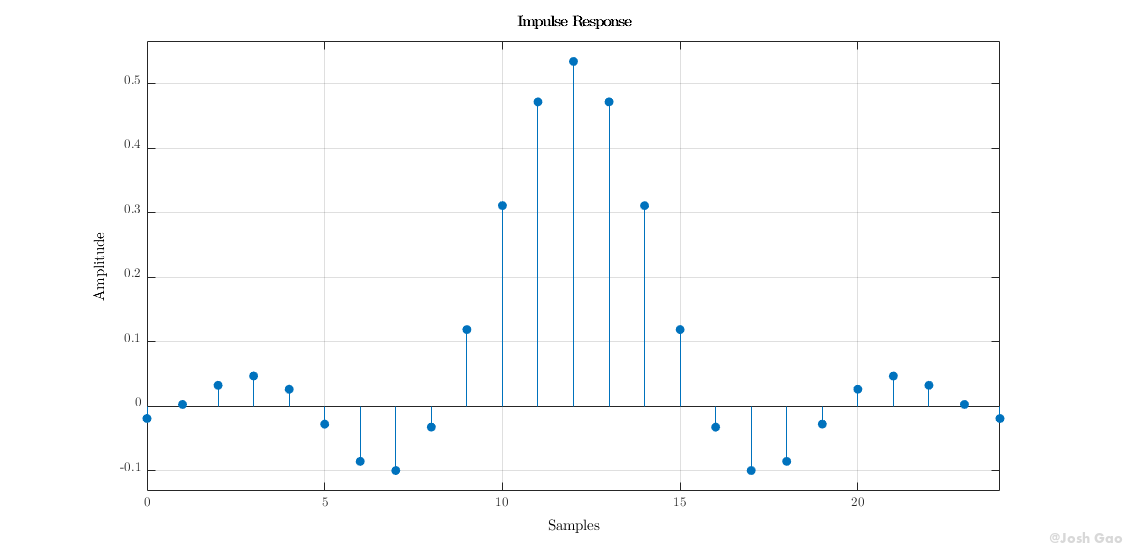
-  <img src="https://josh-blog-1257563604.cos.ap-beijing.myqcloud.com/img/2020-11-25-matlab-rcosdesign/2020-11-25-matlab-rcosdesign-010-DesignASquareRootRaisedCosineFilterExample-01.png?imageMogr2/thumbnail/!100p|watermark/2/text/QEpvc2ggR2Fv/fontsize/15/dissolve/60/gravity/southeast/dx/5/dy/5"/>
-</div>
 
-## 升余弦和根升余弦滤波器的脉冲响应<span id="Examples-02"></span>
+## 升余弦和根升余弦滤波器的脉冲响应<a name="Examples-02"></a>
 
-将升余弦滤波器与根升余弦滤波器进行比较。一个理想的（无限长）升余弦脉冲成型滤波器等效于两个级联的理想的根升余弦滤波器。因此，FIR 升余弦滤波器的脉冲响应应类似于与其自身卷积的根升余弦滤波器的脉冲响应。
+将升余弦滤波器与根升余弦滤波器进行比较。一个理想的（无限长）升余弦脉冲成形滤波器等效于两个级联的理想的根升余弦滤波器。因此，FIR 升余弦滤波器的脉冲响应应类似于与其自身卷积的根升余弦滤波器的脉冲响应。
 
 设计一个衰减为 `0.25` 的升余弦滤波器。指定滤波器有 `4` 个符号，每个符号 `3` 个采样点。
 
-```m
+``` matlab
 rf = 0.25;
 span = 4;
 sps = 3;
@@ -66,24 +63,20 @@ h1 = rcosdesign(rf,span,sps,'normal');
 fvtool(h1,'impulse')
 ```
 
-<div align="center">
+![ ](https://josh-blog-1257563604.cos.ap-beijing.myqcloud.com/img/2020-11-25-matlab-rcosdesign/2020-11-25-matlab-rcosdesign-020-ImpulseResponsesOfNormalAndSquareRootRaisedCosineFiltersExample-01.png?imageMogr2/thumbnail/!100p|watermark/2/text/QEpvc2ggR2Fv/font/YWhyb25iZC50dGY=/fontsize/14/dissolve/20/gravity/southeast/dx/5/dy/5)
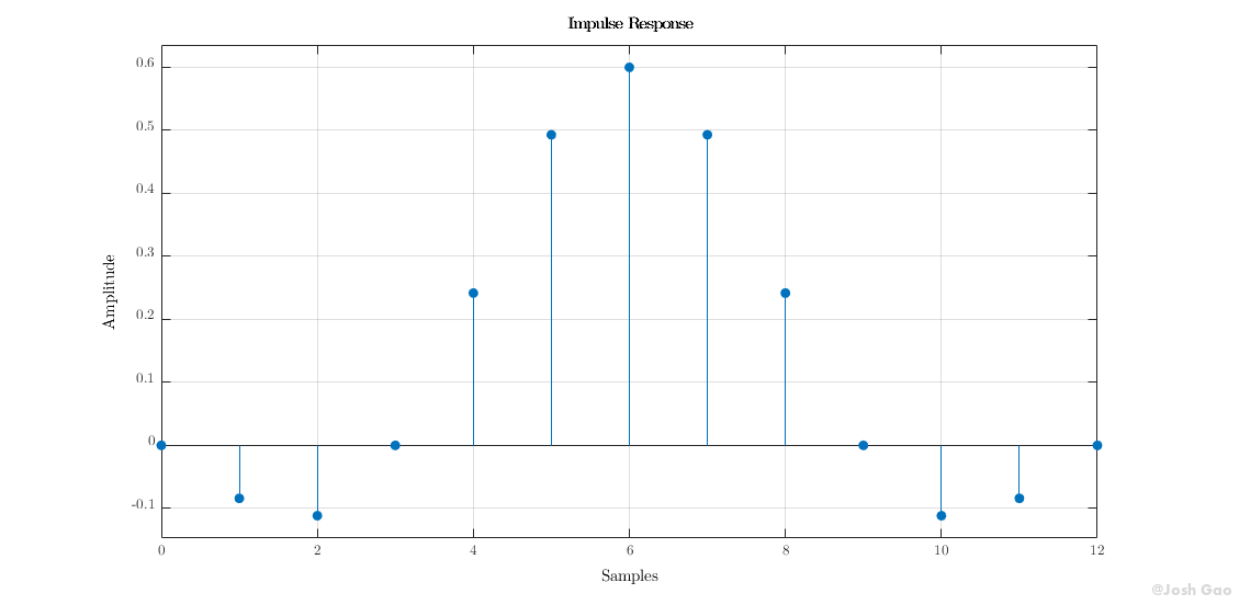
-  <img src="https://josh-blog-1257563604.cos.ap-beijing.myqcloud.com/img/2020-11-25-matlab-rcosdesign/2020-11-25-matlab-rcosdesign-020-ImpulseResponsesOfNormalAndSquareRootRaisedCosineFiltersExample-01.png?imageMogr2/thumbnail/!100p|watermark/2/text/QEpvc2ggR2Fv/fontsize/15/dissolve/60/gravity/southeast/dx/5/dy/5"/>
-</div>
 
 **升余弦滤波器在 `sps` 的整数倍处具有零值点**。因此，它满足无码间串扰（ISI）的 Nyquist 准则。但是，根升余弦滤波器没有这样的特性：
 
-```m
+``` matlab
 h2 = rcosdesign(rf,span,sps,'sqrt');
 fvtool(h2,'impulse')
 ```
 
-<div align="center">
+![ ](https://josh-blog-1257563604.cos.ap-beijing.myqcloud.com/img/2020-11-25-matlab-rcosdesign/2020-11-25-matlab-rcosdesign-030-ImpulseResponsesOfNormalAndSquareRootRaisedCosineFiltersExample-02.png?imageMogr2/thumbnail/!100p|watermark/2/text/QEpvc2ggR2Fv/font/YWhyb25iZC50dGY=/fontsize/14/dissolve/20/gravity/southeast/dx/5/dy/5)
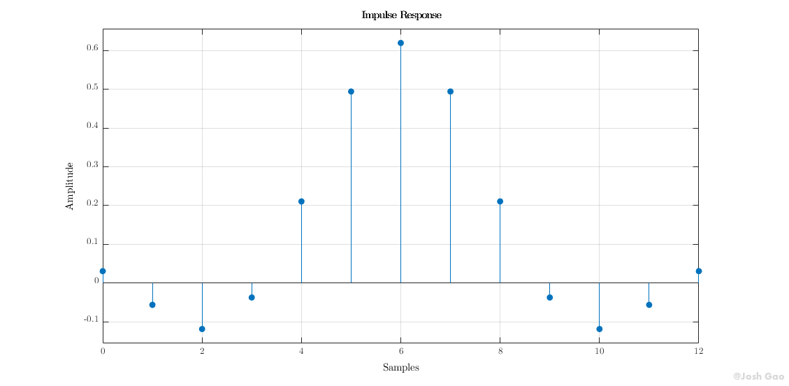
-  <img src="https://josh-blog-1257563604.cos.ap-beijing.myqcloud.com/img/2020-11-25-matlab-rcosdesign/2020-11-25-matlab-rcosdesign-030-ImpulseResponsesOfNormalAndSquareRootRaisedCosineFiltersExample-02.png?imageMogr2/thumbnail/!100p|watermark/2/text/QEpvc2ggR2Fv/fontsize/15/dissolve/60/gravity/southeast/dx/5/dy/5"/>
-</div>
 
 将根升余弦滤波器与自身进行卷积。在最大值处截断脉冲响应，使其长度与 `h1` 相同。使用最大值将响应归一化。然后，将卷积后的根升余弦滤波器与升余弦滤波器进行比较。
 
-```m
+``` matlab
 h3 = conv(h2,h2);
 p2 = ceil(length(h3)/2);
 m2 = ceil(p2-length(h1)/2);
@@ -96,19 +89,17 @@ ylabel('Normalized amplitude')
 legend('h1','h2 * h2')
 ```
 
-<div align="center">
+![ ](https://josh-blog-1257563604.cos.ap-beijing.myqcloud.com/img/2020-11-25-matlab-rcosdesign/2020-11-25-matlab-rcosdesign-040-ImpulseResponsesOfNormalAndSquareRootRaisedCosineFiltersExample-03.png?imageMogr2/thumbnail/!100p|watermark/2/text/QEpvc2ggR2Fv/font/YWhyb25iZC50dGY=/fontsize/14/dissolve/20/gravity/southeast/dx/5/dy/5)
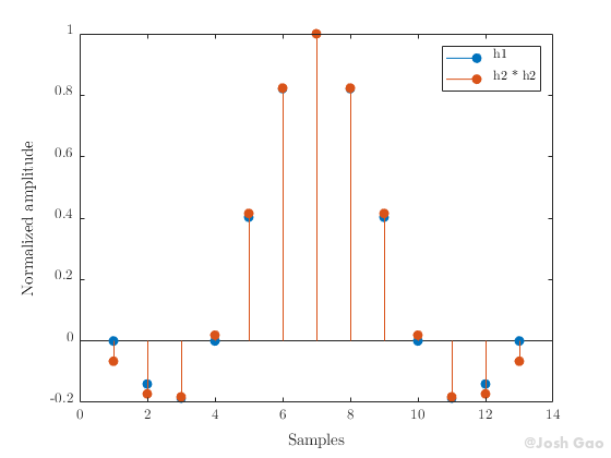
-  <img src="https://josh-blog-1257563604.cos.ap-beijing.myqcloud.com/img/2020-11-25-matlab-rcosdesign/2020-11-25-matlab-rcosdesign-040-ImpulseResponsesOfNormalAndSquareRootRaisedCosineFiltersExample-03.png?imageMogr2/thumbnail/!100p|watermark/2/text/QEpvc2ggR2Fv/fontsize/15/dissolve/60/gravity/southeast/dx/5/dy/5"/>
-</div>
 
 卷积响应的长度是有限的，因此根升余弦滤波器与自身进行卷积得到的结果会与升余弦滤波器不一致。增加 `span` 可以在响应之间获得更紧密的一致性，并更好地符合 Nyquist 准则。
 
-## 将信号通过升余弦滤波器<span id="Examples-03"></span>
+## 将信号通过升余弦滤波器<a name="Examples-03"></a>
 
 本例说明如何将信号通过根升余弦滤波器。
 
 指定滤波器参数。
 
-```m
+``` matlab
 rolloff = 0.25;     % 滚降因子
 span = 6;           % 滤波器宽度（符号数）
 sps = 4;            % 每个符号的样本数
@@ -116,31 +107,31 @@ sps = 4;            % 每个符号的样本数
 
 生成根升余弦滤波器的系数。
 
-```m
+``` matlab
 b = rcosdesign(rolloff, span, sps);
 ```
 
 生成双极性数据向量。
 
-```m
+``` matlab
 d = 2*randi([0 1], 100, 1) - 1;
 ```
 
-上采样并对数据进行滤波以实现脉冲成型。
+上采样并对数据进行滤波以实现脉冲成形。
 
-```m
+``` matlab
 x = upfirdn(d, b, sps);
 ```
 
 添加噪声。
 
-```m
+``` matlab
 r = x + randn(size(x))*0.01;
 ```
 
 对接收到的信号进行滤波和下采样以进行匹配滤波。
 
-```m
+``` matlab
 y = upfirdn(r, b, 1, sps);
 ```
 
@@ -196,6 +187,10 @@ y = upfirdn(r, b, 1, sps);
 >>
 >> 所有输入必须为常数。 如果表达式或变量的值不变，则也允许使用。
 
+# 版本历史
+
+在 R2013b 中推出
+
 # 另请参阅
 
 [`gaussdesign`](https://ww2.mathworks.cn/help/signal/ref/gaussdesign.html)
@@ -204,10 +199,4 @@ y = upfirdn(r, b, 1, sps);
 
 [用 RRC 滤波器进行插值和抽取](https://ww2.mathworks.cn/help/comm/ug/interpolate-and-decimate-using-rrc-filter.html)（Communications Toolbox）
 
-----
+> 原文参考：[https://ww2.mathworks.cn/help/signal/ref/rcosdesign.html](https://ww2.mathworks.cn/help/signal/ref/rcosdesign.html)
-
-在 R2013b 中推出
-
-----
-
-原文参考：[https://ww2.mathworks.cn/help/signal/ref/rcosdesign.html](https://ww2.mathworks.cn/help/signal/ref/rcosdesign.html)

source/_posts/2020-11-26-matlab-gaussdesign.md

@@ -3,19 +3,18 @@ title: MATLAB 函数 —— gaussdesign
 tags:
   - MATLAB
   - 翻译
-  - 成型滤波器
+  - 成形滤波器
   - 滤波器
 categories:
-  - - MATLAB
+  - [MATLAB, 函数用法]
-  - - 翻译
-    - 帮助文档
 mathjax: true
 copyright: true
+comments: true
 abbrlink: a2967b00
 date: 2020-11-26 15:56:26
 ---
 
-`gaussdesign`：高斯 FIR 脉冲成型滤波器设计
+`gaussdesign`：高斯 FIR 脉冲成形滤波器设计
 
 # 语法
 
@@ -25,15 +24,15 @@ date: 2020-11-26 15:56:26
 
 # 说明
 
-`h = gaussdesign(bt,span,sps)` 设计一个低通 FIR 高斯脉冲成型滤波器，并返回滤波器系数向量 `h`。滤波器有 `span` 个符号，每个符号包含 `sps` 个样本。滤波器的阶次，也即 `sps * span` 必须是偶数。[举例](#Examples-01)
+`h = gaussdesign(bt,span,sps)` 设计一个低通 FIR 高斯脉冲成形滤波器，并返回滤波器系数向量 `h`。滤波器有 `span` 个符号，每个符号包含 `sps` 个样本。滤波器的阶次，也即 `sps * span` 必须是偶数。[举例](#Examples-01)
 
 # 示例
 
-## GSM GMSK 数字蜂窝通信系统的高斯滤波器<span id="Examples-01"></span>
+## GSM GMSK 数字蜂窝通信系统的高斯滤波器<a name="Examples-01"></a>
 
 指定用于传输比特位的调制是高斯最小频移键控（GMSK）脉冲。此脉冲的 3-dB 带宽等于比特率的 `0.3` 倍，滤波器的符号数为 `4`，每个符号 `8` 个采样点。
 
-```m
+``` matlab
 bt = 0.3;
 span = 4;
 sps = 8;
@@ -41,9 +40,7 @@ h = gaussdesign(bt,span,sps);
 fvtool(h,'impulse')
 ```
 
-<div align="center">
+![ ](https://josh-blog-1257563604.cos.ap-beijing.myqcloud.com/img/2020-11-26-matlab-gaussdesign/2020-11-26-matlab-gaussdesign-010-GaussianFilterForAGSMGMSKDigitalCellularCommunicationSysExample-01.png?imageMogr2/thumbnail/!100p|watermark/2/text/QEpvc2ggR2Fv/font/YWhyb25iZC50dGY=/fontsize/14/dissolve/20/gravity/southeast/dx/5/dy/5)
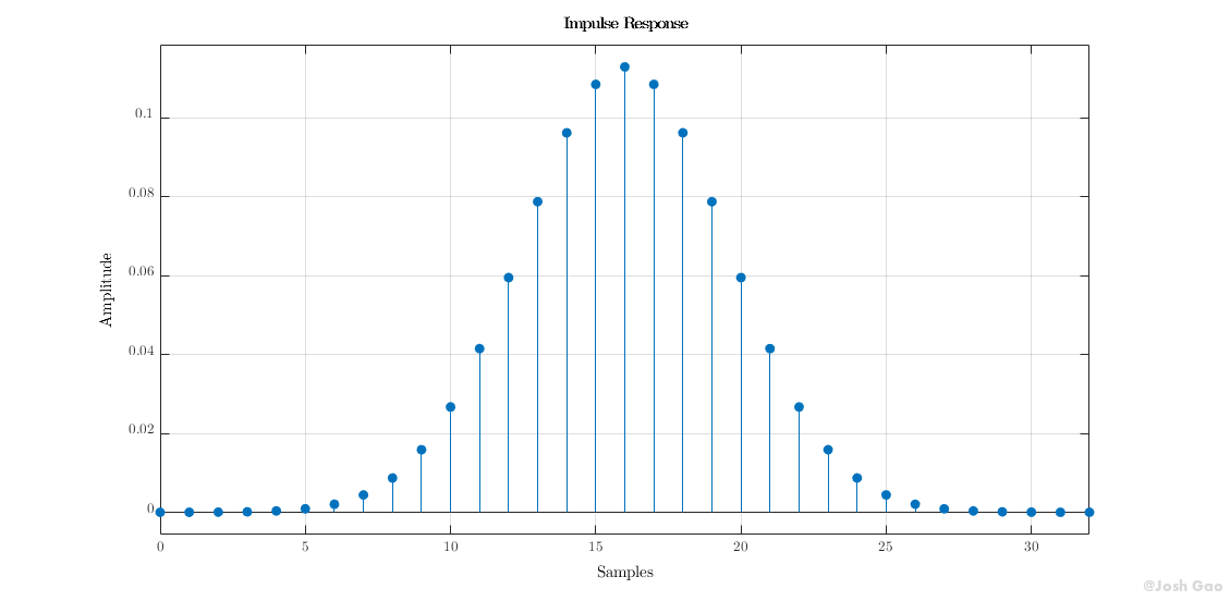
-  <img src="https://josh-blog-1257563604.cos.ap-beijing.myqcloud.com/img/2020-11-26-matlab-gaussdesign/2020-11-26-matlab-gaussdesign-010-GaussianFilterForAGSMGMSKDigitalCellularCommunicationSysExample-01.png?imageMogr2/thumbnail/!100p|watermark/2/text/QEpvc2ggR2Fv/fontsize/15/dissolve/60/gravity/southeast/dx/5/dy/5"/>
-</div>
 
 # 输入参数
 
@@ -69,7 +66,7 @@ fvtool(h,'impulse')
 
 ## `h` - FIR 滤波器系数
 
-高斯脉冲成型滤波器的 FIR 系数，以**行向量**的形式返回。系数已被归一化，因此标称通带增益始终为 1。
+高斯脉冲成形滤波器的 FIR 系数，以**行向量**的形式返回。系数已被归一化，因此标称通带增益始终为 1。
 
 **数据类型**：`double` | `single`
 
@@ -79,14 +76,12 @@ fvtool(h,'impulse')
 
 [2] Rappaport, Theodore S. *Wireless Communications: Principles and Practice.* 2nd Ed. Upper Saddle River, NJ: Prentice Hall, 2002.
 
+# 版本历史
+
+在 R2013b 中推出
+
 # 另请参阅
 
 [`rcosdesign`](https://ww2.mathworks.cn/help/signal/ref/rcosdesign.html)
 
----
-
-在 R2013b 中推出
-
----
-
 原文参考：[https://ww2.mathworks.cn/help/signal/ref/gaussdesign.html](https://ww2.mathworks.cn/help/signal/ref/gaussdesign.html)

source/_posts/2020-11-26-matlab-upsample-spt.md

@@ -5,14 +5,14 @@ tags:
   - 翻译
   - 上采样
 categories:
-  - - MATLAB
+  - [MATLAB, 函数用法]
-  - - 翻译
-    - 帮助文档
 mathjax: true
 copyright: true
+comments: true
 abbrlink: 3a606c9c
 date: 2020-11-26 22:23:39
 ---
+
 `upsample`：将采样率提高整数倍
 
 # 语法
@@ -30,16 +30,16 @@ date: 2020-11-26 22:23:39
 
 # 示例
 
-## 提高采样率<span id="Examples-01"></span>
+## 提高采样率<a name="Examples-01"></a>
 
 将序列的采样率提高 `3` 倍。
 
-```m
+``` matlab 输入
 x = [1 2 3 4];
 y = upsample(x,3)
 ```
 
-```no
+``` plain 输出
 y = 1×12
 
     1     0     0     2     0     0     3     0     0     4     0     0
@@ -47,12 +47,12 @@ y = 1×12
 
 将序列的采样率增加 `3` 倍，并将相位偏移增加 `2`。
 
-```m
+``` matlab 输入
 x = [1 2 3 4];
 y = upsample(x,3,2)
 ```
 
-```no
+``` plain 输出
 y = 1×12
 
     0     0     1     0     0     2     0     0     3     0     0     4     0
@@ -60,14 +60,14 @@ y = 1×12
 
 将矩阵的采样率提高3倍。
 
-```m
+``` matlab 输入
 x = [1 2;
      3 4;
      5 6];
 y = upsample(x,3)
 ```
 
-```no
+``` plain 输出
 y = 9×2
 
     1     2
@@ -115,12 +115,12 @@ y = 9×2
 
 > 使用 MATLAB® Coder™ 生成 C 代码和 C++ 代码。
 
+# 版本历史
+
+在 R2006a 之前推出
+
 # 另请参阅
 
 [`decimate`](https://ww2.mathworks.cn/help/signal/ref/decimate.html) | [`downsample`](https://ww2.mathworks.cn/help/signal/ref/downsample.html) | [`interp`](https://ww2.mathworks.cn/help/signal/ref/interp.html) | [`interp1`](https://ww2.mathworks.cn/help/matlab/ref/interp1.html) | [`resample`](https://ww2.mathworks.cn/help/signal/ref/resample.html) | [`spline`](https://ww2.mathworks.cn/help/matlab/ref/spline.html) | [`upfirdn`](https://ww2.mathworks.cn/help/signal/ref/upfirdn.html)
 
---------------------------------------------------------------------------------
+> 原文参考：[https://ww2.mathworks.cn/help/signal/ref/upsample.html](https://ww2.mathworks.cn/help/signal/ref/upsample.html)
-在 R2006a 之前推出
-
---------------------------------------------------------------------------------
-原文参考：[https://ww2.mathworks.cn/help/signal/ref/upsample.html](https://ww2.mathworks.cn/help/signal/ref/upsample.html)

source/_posts/2020-11-27-hexo-next-busuanzi-issues.md

@@ -5,8 +5,10 @@ tags:
   - Hexo
   - Next
 categories:
-  - [Blog, Hexo, Next]
+  - [Blog, Hexo]
 abbrlink: e96c9b26
+copyright: true
+comments: true
 date: 2020-11-27 11:15:21
 ---
 
@@ -45,23 +47,15 @@ busuanzi_count:
 
 添加 Live2D 前的不蒜子显示情况如下。
 
-<div align="center">
+![添加 Live2D 前单篇博客的不蒜子显示情况](https://josh-blog-1257563604.cos.ap-beijing.myqcloud.com/img/2020-11-27-hexo-next-busuanzi-issues/2020-11-27-hexo-next-busuanzi-issues-010-Live2D-01.png?imageMogr2/thumbnail/!100p|watermark/2/text/QEpvc2ggR2Fv/font/YWhyb25iZC50dGY=/fontsize/14/dissolve/20/gravity/southeast/dx/5/dy/5)
-  <img src="https://josh-blog-1257563604.cos.ap-beijing.myqcloud.com/img/2020-11-27-hexo-next-busuanzi-issues/2020-11-27-hexo-next-busuanzi-issues-010-Live2D-01.png?imageMogr2/thumbnail/!100p|watermark/2/text/QEpvc2ggR2Fv/fontsize/15/dissolve/60/gravity/southeast/dx/5/dy/5"/>
-</div>
 
-<div align="center">
+![添加 Live2D 前网站的不蒜子显示情况](https://josh-blog-1257563604.cos.ap-beijing.myqcloud.com/img/2020-11-27-hexo-next-busuanzi-issues/2020-11-27-hexo-next-busuanzi-issues-020-Live2D-02.png?imageMogr2/thumbnail/!100p|watermark/2/text/QEpvc2ggR2Fv/font/YWhyb25iZC50dGY=/fontsize/14/dissolve/20/gravity/southeast/dx/5/dy/5)
-  <img src="https://josh-blog-1257563604.cos.ap-beijing.myqcloud.com/img/2020-11-27-hexo-next-busuanzi-issues/2020-11-27-hexo-next-busuanzi-issues-020-Live2D-02.png?imageMogr2/thumbnail/!100p|watermark/2/text/QEpvc2ggR2Fv/fontsize/15/dissolve/60/gravity/southeast/dx/5/dy/5"/>
-</div>
 
 添加 Live2D 后，不蒜子在页面中不显示。
 
-<div align="center">
+![添加 Live2D 后单篇博客的不蒜子显示情况](https://josh-blog-1257563604.cos.ap-beijing.myqcloud.com/img/2020-11-27-hexo-next-busuanzi-issues/2020-11-27-hexo-next-busuanzi-issues-030-Live2D-03.png?imageMogr2/thumbnail/!100p|watermark/2/text/QEpvc2ggR2Fv/font/YWhyb25iZC50dGY=/fontsize/14/dissolve/20/gravity/southeast/dx/5/dy/5)
-  <img src="https://josh-blog-1257563604.cos.ap-beijing.myqcloud.com/img/2020-11-27-hexo-next-busuanzi-issues/2020-11-27-hexo-next-busuanzi-issues-030-Live2D-03.png?imageMogr2/thumbnail/!100p|watermark/2/text/QEpvc2ggR2Fv/fontsize/15/dissolve/60/gravity/southeast/dx/5/dy/5"/>
-</div>
 
-<div align="center">
+![添加 Live2D 后网站的不蒜子显示情况](https://josh-blog-1257563604.cos.ap-beijing.myqcloud.com/img/2020-11-27-hexo-next-busuanzi-issues/2020-11-27-hexo-next-busuanzi-issues-040-Live2D-04.png?imageMogr2/thumbnail/!100p|watermark/2/text/QEpvc2ggR2Fv/font/YWhyb25iZC50dGY=/fontsize/14/dissolve/20/gravity/southeast/dx/5/dy/5)
-  <img src="https://josh-blog-1257563604.cos.ap-beijing.myqcloud.com/img/2020-11-27-hexo-next-busuanzi-issues/2020-11-27-hexo-next-busuanzi-issues-040-Live2D-04.png?imageMogr2/thumbnail/!100p|watermark/2/text/QEpvc2ggR2Fv/fontsize/15/dissolve/60/gravity/southeast/dx/5/dy/5"/>
-</div>
 
 ## 问题原因
 
@@ -91,9 +85,7 @@ busuanzi_count:
 
 在网页生成引擎中修改代码，去掉不蒜子部分的 `id` 和 `style` 属性，重新生成网页即可解决该问题。若将 `class` 属性一并删除，会导不蒜子部分和前面的其他显示部分缺少分隔符，如下图。
 
-<div align="center">
+![ ](https://josh-blog-1257563604.cos.ap-beijing.myqcloud.com/img/2020-11-27-hexo-next-busuanzi-issues/2020-11-27-hexo-next-busuanzi-issues-050-Delimeter-01.png?imageMogr2/thumbnail/!100p|watermark/2/text/QEpvc2ggR2Fv/font/YWhyb25iZC50dGY=/fontsize/14/dissolve/20/gravity/southeast/dx/5/dy/5)
-  <img src="https://josh-blog-1257563604.cos.ap-beijing.myqcloud.com/img/2020-11-27-hexo-next-busuanzi-issues/2020-11-27-hexo-next-busuanzi-issues-050-Delimeter-01.png?imageMogr2/thumbnail/!100p|watermark/2/text/QEpvc2ggR2Fv/fontsize/15/dissolve/60/gravity/southeast/dx/5/dy/5"/>
-</div>
 
 具体需要修改两个文件，`next/layout/_third-party/statistics/busuanzi-counter.swig` 中修改的是网页页脚部分的不蒜子显示，`next/layout/_macro/post.swig` 中修改的博客文章阅览数的不蒜子显示。
 

source/_posts/2020-11-27-josh-verilog-part-1.md

@@ -9,12 +9,10 @@ tags:
   - RTL
   - 寄存器传输级
 categories:
-  - [Verilog, Verilog 简介]
   - [Josh 的学习笔记, Verilog]
 mathjax: true
 comments: true
 copyright: true
-sticky: false
 toc:
   enable: true
   number: false
@@ -106,9 +104,7 @@ Verilog 语言是根据 C 语言发明而来的，因此 Verilog 具备了 C 语
 
 HDL 的基本功能就是有效地描述并仿真硬件系统。在此部分，抛开具体的 PLD 或 ASIC 设计流程，从 HDL 语言层次入手，分析典型的 HDL 设计与验证流程。基于 HDL 的设计、仿真流程如下图所示。图中，虚线框表示的步骤可以根据项目的复杂度省略，而实线框表示的步骤为必须执行的步骤。
 
-<div align="center">
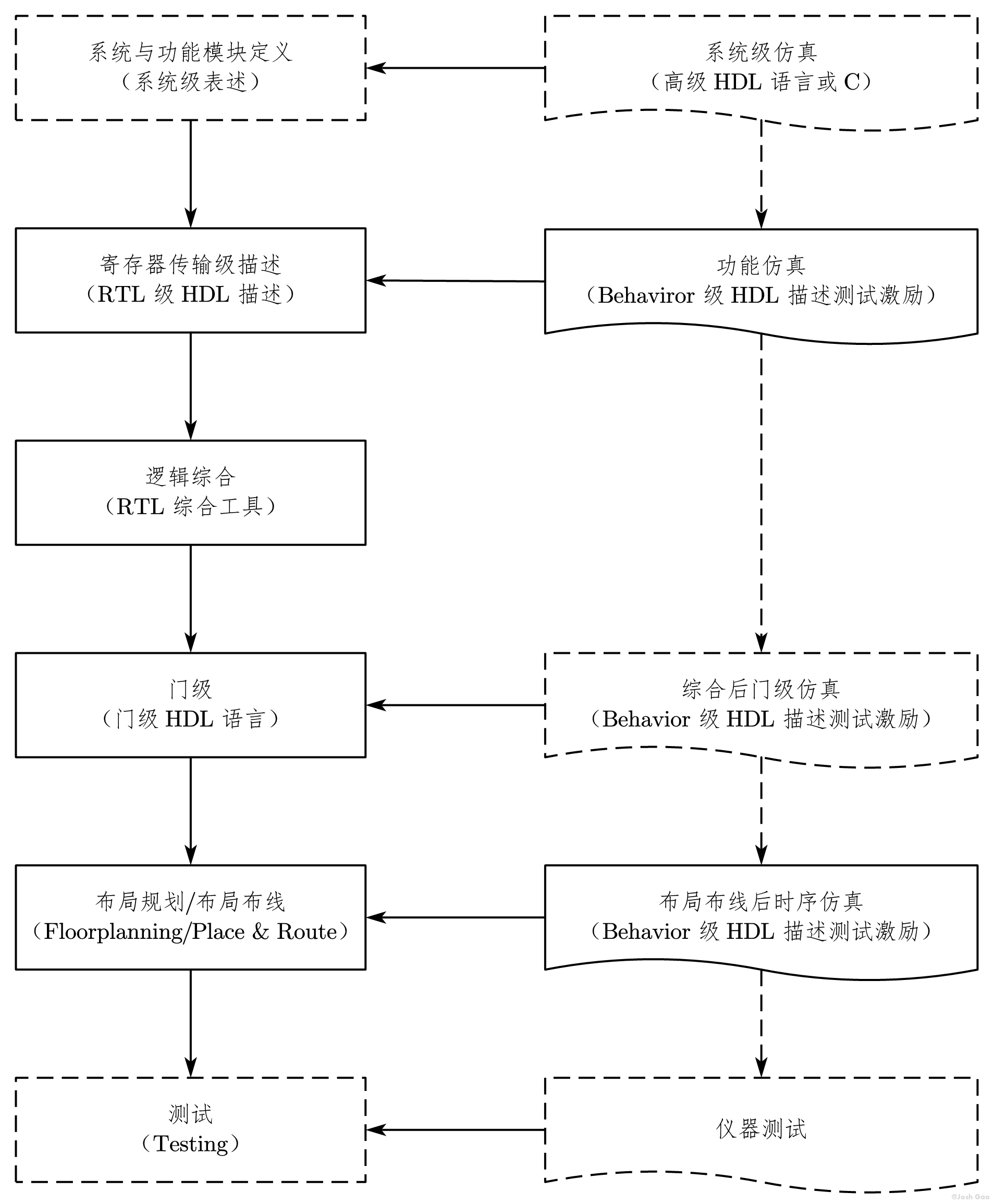+![基于 HDL 的设计、仿真流程](https://josh-blog-1257563604.cos.ap-beijing.myqcloud.com/img/2020-11-27-josh-verilog-part-1/2020-11-27-josh-verilog-part-1-010-DesignSimulationFlowChartBasedonHDL.png?imageMogr2/thumbnail/!100p|watermark/2/text/QEpvc2ggR2Fv/font/YWhyb25iZC50dGY=/fontsize/14/dissolve/20/gravity/southeast/dx/5/dy/5){width=800px}
-  <img src="https://josh-blog-1257563604.cos.ap-beijing.myqcloud.com/img/2020-11-27-josh-verilog-part-1/2020-11-27-josh-verilog-part-1-010-DesignSimulationFlowChartBasedonHDL.png!800px"/>
-</div>
 
 下面对一些关键设计步骤与概念进行展开。
 

source/_posts/2020-11-27-matlab-awgn.md

@@ -5,13 +5,11 @@ tags:
   - 翻译
   - 高斯白噪声
 categories:
-  - - MATLAB
+  - [MATLAB, 函数用法]
-  - - 翻译
+  - [信号处理, 噪声]
-    - 帮助文档
-  - - 信号处理
-    - 噪声
 mathjax: true
 copyright: true
+comments: true
 abbrlink: 2f6db45b
 date: 2020-11-27 01:15:12
 ---
@@ -49,22 +47,20 @@ date: 2020-11-27 01:15:12
 
 创建一个锯齿波。
 
-```m
+``` matlab
 t = (0:0.1:10)';
 x = sawtooth(t);
 ```
 
 添加高斯白噪声并绘制结果。
 
-```m
+``` matlab
 y = awgn(x,10,'measured');
 plot(t,[x y])
 legend('Original Signal','Signal with AWGN')
 ```
 
-<div align="center">
+![ ](https://josh-blog-1257563604.cos.ap-beijing.myqcloud.com/img/2020-11-27-matlab-awgn/2020-11-27-matlab-awgn-010-AddAWGNToSawtoothSignalExample-01.png?imageMogr2/thumbnail/!100p|watermark/2/text/QEpvc2ggR2Fv/font/YWhyb25iZC50dGY=/fontsize/14/dissolve/20/gravity/southeast/dx/5/dy/5)
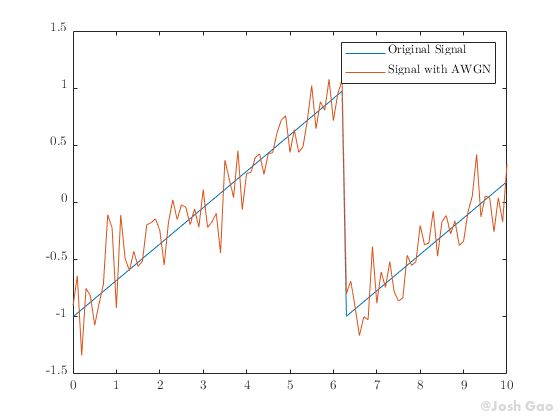
-  <img src="https://josh-blog-1257563604.cos.ap-beijing.myqcloud.com/img/2020-11-27-matlab-awgn/2020-11-27-matlab-awgn-010-AddAWGNToSawtoothSignalExample-01.png?imageMogr2/thumbnail/!100p|watermark/2/text/QEpvc2ggR2Fv/fontsize/15/dissolve/60/gravity/southeast/dx/5/dy/5"/>
-</div>
 
 ## AWGN 信道中的常规 QAM 调制<span id="Examples-02"></span>
 
@@ -72,32 +68,32 @@ legend('Original Signal','Signal with AWGN')
 
 根据电话线调制解调器的 V.29 标准创建一个 16-QAM 星座。
 
-```m
+``` matlab
 c = [-5 -5i 5 5i -3 -3-3i -3i 3-3i 3 3+3i 3i -3+3i -1 -1i 1 1i];
 M = length(c);
 ```
 
 生成随机符号。
 
-```m
+``` matlab
 data = randi([0 M-1],2000,1);
 ```
 
 使用 `genqammod` 函数调制数据。由于星座图不是矩形，因此必须进行常规 QAM 调制。
 
-```m
+``` matlab
 modData = genqammod(data,c);
 ```
 
 使信号通过具有 20 dB 信噪比（SNR）的 AWGN 信道。
 
-```m
+``` matlab
 rxSig = awgn(modData,20,'measured');
 ```
 
 显示接收信号的星座图和参考星座图。
 
-```m
+``` matlab
 h = scatterplot(rxSig);
 hold on
 scatterplot(c,[],[],'r*',h)
@@ -105,31 +101,29 @@ grid
 hold off
 ```
 
-<div align="center">
+![ ](https://josh-blog-1257563604.cos.ap-beijing.myqcloud.com/img/2020-11-27-matlab-awgn/2020-11-27-matlab-awgn-020-GeneralQAMModulationInAnAWGNChannelExample-01.png?imageMogr2/thumbnail/!100p|watermark/2/text/QEpvc2ggR2Fv/fontsize/15/dissolve/60/gravity/southeast/dx/5/dy/5)
-  <img src="https://josh-blog-1257563604.cos.ap-beijing.myqcloud.com/img/2020-11-27-matlab-awgn/2020-11-27-matlab-awgn-020-GeneralQAMModulationInAnAWGNChannelExample-01.png?imageMogr2/thumbnail/!100p|watermark/2/text/QEpvc2ggR2Fv/fontsize/15/dissolve/60/gravity/southeast/dx/5/dy/5"/>
-</div>
 
 使用 `genqamdemod` 函数解调接收到的信号。计算误符号数和误符号率。
 
-```m
+``` matlab 输入
 demodData = genqamdemod(rxSig,c);
 [numErrors,ser] = symerr(data,demodData)
 ```
 
-```no
+``` plain 输出
 numErrors = 1
 ser = 5.0000e-04
 ```
 
 使用具有 10 dB SNR 的 AWGN 信道重复传输和解调过程。计算降低 SNR 后的误符号率。不出所料，当 SNR 降低时，性能会下降。
 
-```m
+``` matlab 输入
 rxSig = awgn(modData,10,'measured');
 demodData = genqamdemod(rxSig,c);
 [numErrors,ser] = symerr(data,demodData)
 ```
 
-```no
+``` plain 输出
 numErrors = 462
 ser = 0.2310
 ```
@@ -140,7 +134,7 @@ ser = 0.2310
 
 将 X 的功率指定为 0 dBW，添加噪声以产生 10 dB 的 SNR，并利用本地随机流。
 
-```m
+``` matlab 输入
 S = RandStream('mt19937ar','Seed',5489);
 sigin = sqrt(2)*sin(0:pi/8:6*pi);
 sigout1 = awgn(sigin,10,0,S);
@@ -148,25 +142,25 @@ sigout1 = awgn(sigin,10,0,S);
 
 将 AWGN 添加到 `sigin`。 使用 [`isequal`](https://ww2.mathworks.cn/help/matlab/ref/isequal.html) 比较 `sigout1` 和 `sigout2`。 当不重置随机流时，输出不相等。
 
-```m
+``` matlab 输入
 sigout2 = awgn(sigin,10,0,S);
 isequal(sigout1,sigout2)
 ```
 
-```no
+``` plain 输出
 ans = logical
    0
 ```
 
 重置随机流对象，将对象置为初始状态，然后再将 AWGN 添加到 `sigout1`。将 AWGN 添加到 `sigin` 并将 `sigout1` 与 `sigout3` 比较。 重置随机流后，输出相等。
 
-```m
+``` matlab 输入
 reset(S);
 sigout3 = awgn(sigin,10,0,S);
 isequal(sigout1,sigout3)
 ```
 
-```no
+``` plain 输出
 ans = logical
    1
 ```
@@ -260,6 +254,10 @@ ans = logical
 >>
 >> 支持代码生成，但包括 [`RandStream`](https://ww2.mathworks.cn/help/matlab/ref/randstream.html) 对象的语法除外。
 
+# 版本历史
+
+在 R2006a 之前推出
+
 # 另请参阅
 
 ## 函数
@@ -274,8 +272,4 @@ ans = logical
 
 [AWGN Channel Noise Level](https://ww2.mathworks.cn/help/comm/ug/awgn-channel.html#a1071501088)
 
---------------------------------------------------------------------------------
-在 R2006a 之前推出
-
---------------------------------------------------------------------------------
 原文参考：[https://ww2.mathworks.cn/help/comm/ref/awgn.html](https://ww2.mathworks.cn/help/comm/ref/awgn.html)

source/_posts/2020-11-28-josh-verilog-part-2.md

@@ -8,7 +8,6 @@ tags:
   - 自底向上
   - Verilog 语法
 categories:
-  - [Verilog, Verilog 语法]
   - [Josh 的学习笔记, Verilog]
 mathjax: true
 comments: true
@@ -53,9 +52,7 @@ EDA 行业的先行者们发明了 Verilog 硬件描述语言，其最根本的
 
 <a name="JoshVerilog模块"></a>首先看一个简单的如下图所示的电路（模块）：JoshVerilog。它可以是一个独立的设计，也可以是更大的系统的一个组成部分。
 
-<div align="center">
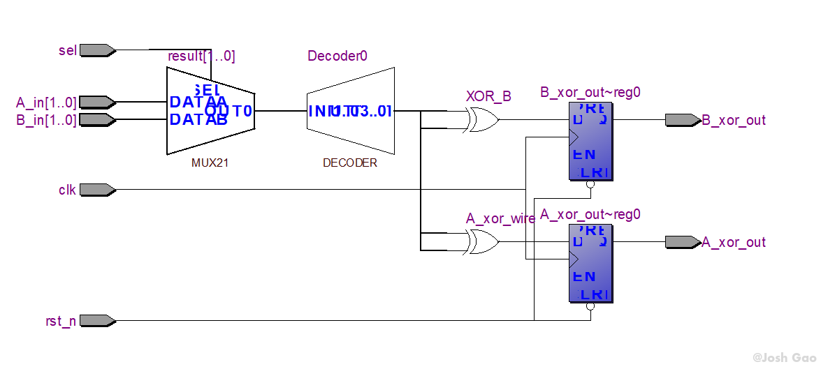+![ ](https://josh-blog-1257563604.cos.ap-beijing.myqcloud.com/img/2020-11-28-josh-verilog-part-2/2020-11-28-josh-verilog-part-2-010-JoshVerilog.png?imageMogr2/thumbnail/!100p|watermark/2/text/QEpvc2ggR2Fv/font/YWhyb25iZC50dGY=/fontsize/18/dissolve/20/gravity/southeast/dx/5/dy/5){width=800px}
-  <img src="https://josh-blog-1257563604.cos.ap-beijing.myqcloud.com/img/2020-11-28-josh-verilog-part-2/2020-11-28-josh-verilog-part-2-010-JoshVerilog.png!700px"/>
-</div>
 
 该电路首先在两个 2 位的输入数据 `A_in[1:0]` 的和 `B_in[1:0]` 之间，由 `sel` 信号做二选一。后面是一个 2-4 译码电路，将输入的信号 `result[1:0]`解析成 `eq0`、`eql`、`eq2` 和 `eq3` 这4个信号，它们同时只有一个为 1。
 
@@ -63,7 +60,7 @@ EDA 行业的先行者们发明了 Verilog 硬件描述语言，其最根本的
 
 **这些电路单元都是同时并行工作的，相互之间并没有先后顺序关系，这一点与软件设计程序很不一样。**
 
-下面具体分析 [JoshVerilog 模块](#JoshVerilog模块)的电路功能。源代码如下。
+下面具体分析 [JoshVerilog 模块](#JoshVerilog模块) 的电路功能。源代码如下。
 
 <a name="JoshVerilog代码"></a>
 

source/_posts/2020-11-30-josh-verilog-part-3.md

@@ -8,7 +8,6 @@ tags:
   - 设计层次
   - Verilog 语法
 categories:
-  - [Verilog, Verilog 设计]
   - [Josh 的学习笔记, Verilog]
 mathjax: true
 comments: true

source/_posts/2020-12-02-josh-verilog-part-4.md

@@ -21,7 +21,6 @@ tags:
   - 异步复位
   - 条件语句
 categories:
-  - [Verilog]
   - [Josh 的学习笔记, Verilog]
 abbrlink: ecb88422
 date: 2020-12-02 01:05:32

source/_posts/2020-12-05-josh-verilog-part-5.md

@@ -19,9 +19,7 @@ tags:
   - 速度
   - 面积
 categories:
-  - - Verilog
+  - [Josh 的学习笔记, Verilog]
-  - - Josh 的学习笔记
-    - Verilog
 abbrlink: 53b8b42e
 date: 2020-12-05 00:46:00
 ---

source/_posts/2021-12-08-josh-msp-part-1.md

@@ -14,7 +14,7 @@ tags:
   - 抽样率转换
   - 抽取
   - 内插
-  - 分数被抽样
+  - 分数倍抽样
 categories:
   - - Josh 的学习笔记
     - 多抽样率信号处理
@@ -30,11 +30,11 @@ date: 2021-12-08 15:28:38
 - 如何实现分数倍抽样率转换？
 - 如何利用 MATLAB 实现抽样率转换？
 
-  多抽样率信号处理的研究对象是不同抽样率[^ChineseofSampling]下的信号，其中抽样率转换 (Sampling Rate Conversion, SRC) 是核心问题之一。早期的抽样率转换通常采用模拟方法，即将给定的抽样信号通过数模转换器 (Digital-to-Analog Converter, DAC) 转换成模拟信号 (连续时间信号)，再对该模拟信号进行新的抽样，经模数转换器 (Analog-to-Digital Converter, DAC) 得到所需的抽样信号。而随着数字电路的普及和数字信号处理技术的发展，采用数字方法，即直接在离散时间域上完成抽样率转换已成为当前的主要方式。相比于模拟方法，数字方法不需要进行D/A和A/D转换，降低了系统的复杂度，同时避免了由量化、编码等过程产生的失真问题。
+  多抽样率信号处理的研究对象是不同抽样率[^SamplingRate]下的信号，其中抽样率转换 (Sampling Rate Conversion, SRC) 是核心问题之一。早期的抽样率转换通常采用模拟方法，即将给定的抽样信号通过数模转换器 (Digital-to-Analog Converter, DAC) 转换成模拟信号 (连续时间信号)，再对该模拟信号进行新的抽样，经模数转换器 (Analog-to-Digital Converter, DAC) 得到所需的抽样信号。而随着数字电路的普及和数字信号处理技术的发展，采用数字方法，即直接在离散时间域上完成抽样率转换已成为当前的主要方式。相比于模拟方法，数字方法不需要进行D/A和A/D转换，降低了系统的复杂度，同时避免了由量化、编码等过程产生的失真问题。
 
   本文首先回顾采样的概念；随后介绍抽样率转换的两个基本运算单元，即抽取和内插；进而讨论如何利用抽取和内插实现分数倍抽样率转换；最后介绍抽样率转换在 MATLAB 上的实现。
 
-[^ChineseofSampling]: 又称采样率，在本文中，“采样”与“抽样”涵义相同，两者经常交换使用。
+[^SamplingRate]: 又称采样率，在本文中，“采样”与“抽样”涵义相同，两者经常交换使用。
 
 <!-- more -->
 
@@ -66,18 +66,17 @@ $$\begin{equation}
 
 对上式作傅里叶变换，记采样信号的频谱为 $X_s\left( j\Omega \right)$，原始信号的频谱为 $X_c\left( j\Omega \right)$，同时注意到脉冲序列的傅里叶变换依然是脉冲序列，根据卷积定理可知，采样信号与原始信号的频谱具有如下关系：
 
-$$\begin{equation} \label{1}
+$$\begin{equation} \label{Relationship between the spectrum of the sampled signal and the original signal}
 X_s\left( j\Omega \right) =\frac{1}{2\pi}X_c\left( j\Omega \right) \ast \frac{2\pi}{T}\sum_{n=-\infty}^{\infty}{\delta \left( \Omega -n\Omega _s \right)}=\frac{1}{T}\sum_{n=-\infty}^{\infty}{X_c\left( j\left( \Omega -\Omega _s \right) \right)}
 \end{equation}$$
 
 其中 $\Omega_s = \displaystyle\frac{2\pi}{T}=2\pi F_s$ 为采样角频率 (亦简称为采样率) 。
 
-&emsp;&emsp;式 $\eqref{1}$ 说明，采样信号的频谱是将原始信号频谱以 $\Omega_s$ 进行周期延拓，且幅度变为原来的 $1/T$，[图 1.1](#图1.1) 给出了该过程的示意图。显然，若采样率过低则会造成相邻周期的频谱交叠在一起产生失真，这种现象称为混叠 (aliasing)。为避免混叠，采样率应大于信号最高频率的 2 倍。在此条件下，通过适当选取一个低通滤波器，可以从采样信号的频谱恢复出原始信号的频谱。这就是著名的 Nyquist-Shannon 采样定理。
+&emsp;&emsp;式 $\eqref{Relationship between the spectrum of the sampled signal and the original signal}$ 说明，采样信号的频谱是将原始信号频谱以 $\Omega_s$ 进行周期延拓，且幅度变为原来的 $1/T$，[图 1.1](#图1.1) 给出了该过程的示意图。显然，若采样率过低则会造成相邻周期的频谱交叠在一起产生失真，这种现象称为混叠 (aliasing)。为避免混叠，采样率应大于信号最高频率的 2 倍。在此条件下，通过适当选取一个低通滤波器，可以从采样信号的频谱恢复出原始信号的频谱。这就是著名的 Nyquist-Shannon 采样定理。
 
-<span id="图1.1"></span>
+<a id="图1.1"></a>
-<div align="center">
+
-  <img src="https://josh-blog-1257563604.cos.ap-beijing.myqcloud.com/img/2021-12-08-josh-msp-part-1/2021-12-08-josh-msp-part-1-010-RelationshipBetweenSampledSignalandAnalogSignal.png" width=500px alt="图1.1 采样信号与模拟信号的关系"/>
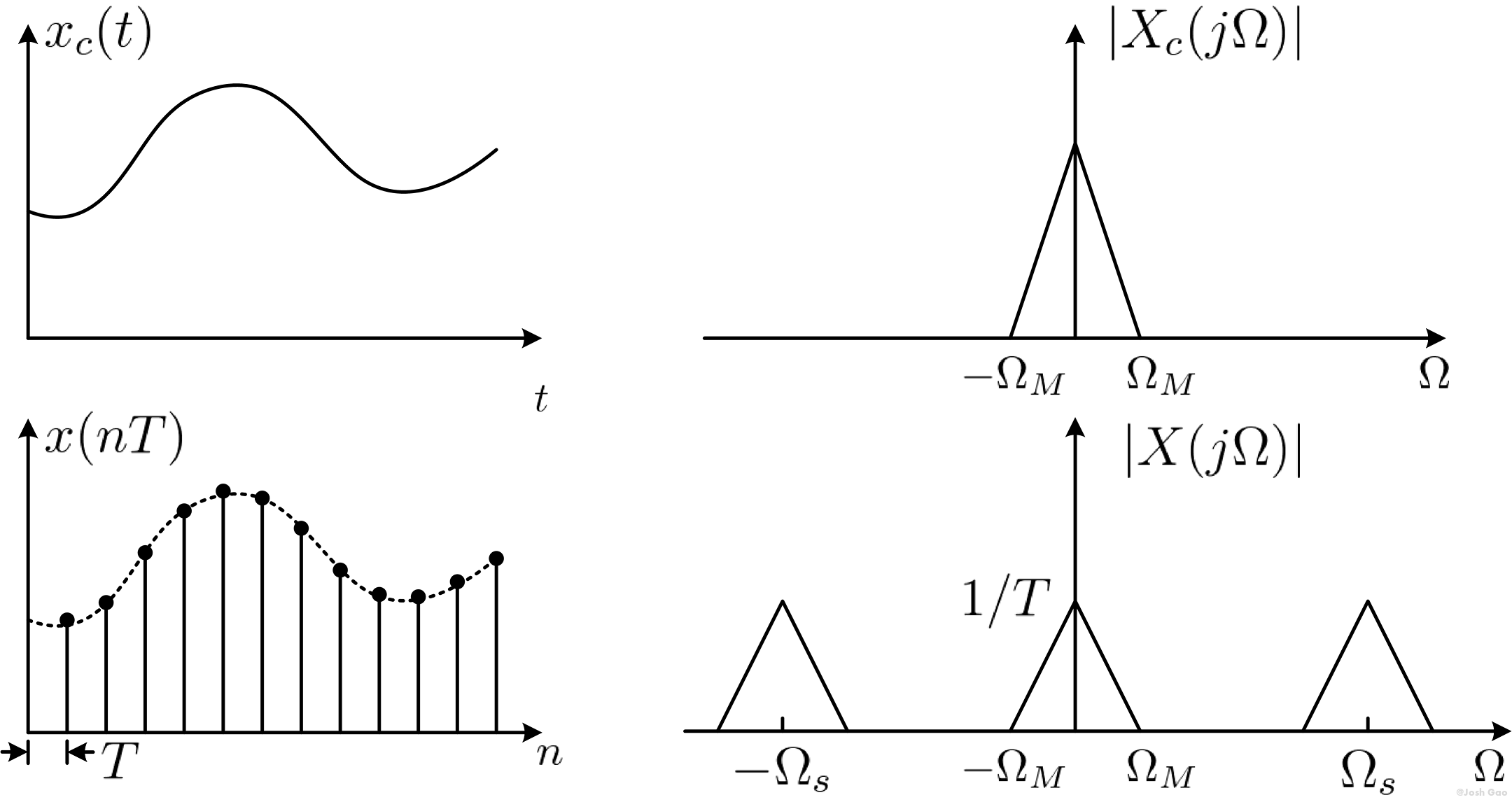+![图1.1 采样信号与模拟信号的关系](https://josh-blog-1257563604.cos.ap-beijing.myqcloud.com/img/2021-12-08-josh-msp-part-1/2021-12-08-josh-msp-part-1-010-RelationshipBetweenSampledSignalandAnalogSignal.png?imageMogr2/thumbnail/!100p|watermark/2/text/QEpvc2ggR2Fv/font/YWhyb25iZC50dGY=/fontsize/14/dissolve/20/gravity/southeast/dx/5/dy/5){width=500px}
-</div>
 
 **定理 1.1 (Nyquist-Shannon 采样定理)** 设 $x\left(t\right)$ 是带限信号，频带范围为 $\left(-\Omega_M,\Omega_M\right)$。如果采样率满足
 
@@ -133,10 +132,9 @@ y_D\left( nT_2 \right) =x\left( nDT_1 \right)
 
 其中 $T_1$、$T_2$ 分别为抽取前后的采样间隔，且 $T_2 = DT_1$。[图 1.2(a)](#图1.2) 给出了 $D=3$ 时抽取过程的示意图。
 
-<span id="图1.2"></span>
+<a id="图1.2"></a>
-<div align="center">
+
-  <img src="https://josh-blog-1257563604.cos.ap-beijing.myqcloud.com/img/2021-12-08-josh-msp-part-1/2021-12-08-josh-msp-part-1-020-DecimationDemostration.png" width=500px alt="图1.2 抽取"/>
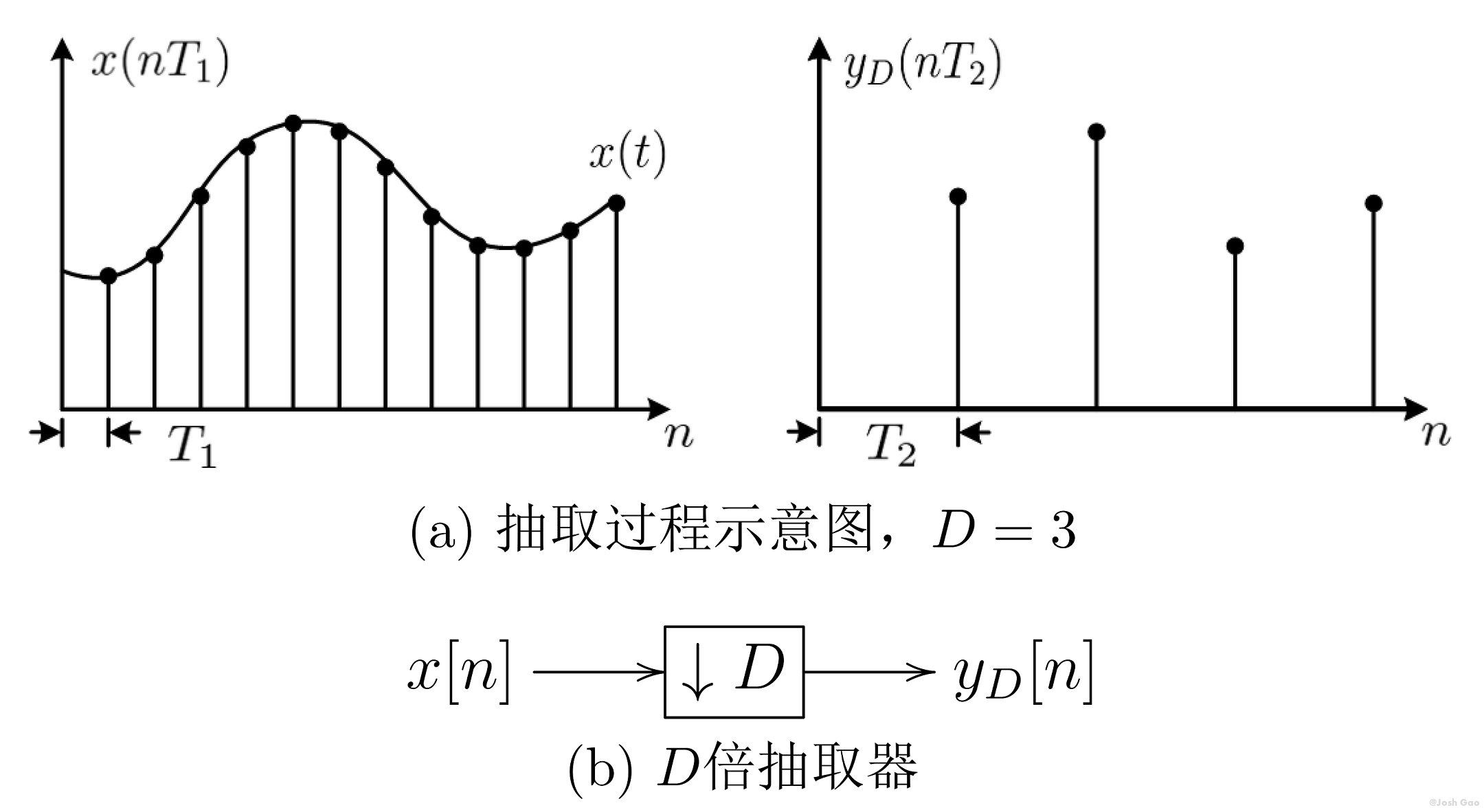+![图1.2 抽取](https://josh-blog-1257563604.cos.ap-beijing.myqcloud.com/img/2021-12-08-josh-msp-part-1/2021-12-08-josh-msp-part-1-020-DecimationDemostration.png?imageMogr2/thumbnail/!100p|watermark/2/text/QEpvc2ggR2Fv/font/YWhyb25iZC50dGY=/fontsize/14/dissolve/20/gravity/southeast/dx/5/dy/5){width=500px}
-</div>
 
 &emsp;&emsp;上述关系也可以简记为
 

source/_posts/2022-05-30-josh-systemverilog-1.md

@@ -2,7 +2,7 @@
 title: 'Josh''s Notes: SystemVerilog 验证 (Part 1 — 验证导论)'
 mathjax: true
 comments: true
-copyright: false
+copyright: true
 sticky: false
 toc:
   enable: true

source/_posts/2022-05-31-josh-systemverilog-2.md

@@ -2,7 +2,7 @@
 title: 'Josh''s Notes: SystemVerilog 验证 (Part 2 — 数据类型)'
 mathjax: true
 comments: true
-copyright: false
+copyright: true
 sticky: false
 toc:
   enable: true

source/_posts/2022-06-02-josh-systemverilog-3.md

@@ -2,7 +2,7 @@
 title: 'Josh''s Notes: SystemVerilog 验证 (Part 3 — 过程语句和子程序)'
 mathjax: true
 comments: true
-copyright: false
+copyright: true
 sticky: false
 toc:
   enable: true

source/_posts/2023-04-08-oxford-5000-pitch.md

@@ -4,7 +4,7 @@ tags:
   - 牛津5000
   - 英语词汇
 comments: true
-copyright: false
+copyright: true
 toc:
   enable: true
   number: true
@@ -34,6 +34,8 @@ date: 2023-04-08 00:04:11
 
    \[countable\] an area of ground specially prepared and marked for playing a sports game
 
+   <!-- more -->
+
    - *a **football pitch*** 足球场
    - *a cricket/rugby/hockey pitch* 板球/橄榄球/曲棍球场
    - *an artificial pitch* 人造沥青
@@ -70,8 +72,6 @@ date: 2023-04-08 00:04:11
 
    {% endnote %}
 
-<!-- more -->
-
 ### {% label primary@of sound 声音 %}
 
 2. [singular, uncountable] how high or low a sound is, especially a musical note（尤指乐音的）音高

source/_posts/2023-04-09-oxford-5000-a-an.md

@@ -4,7 +4,7 @@ tags:
   - 牛津5000
   - 英语词汇
 comments: true
-copyright: false
+copyright: true
 toc:
   enable: true
   number: true
@@ -36,6 +36,8 @@ date: 2023-04-09 00:37:24
 
 1. **{% label @A1 %}** used before countable or singular nouns referring to people or things that have not already been mentioned（用于可数名词或单数名词前，表示未曾提到的）一（人、事、物）
 
+   <!-- more -->
+
    - *a man/horse/unit* 一个人；一匹马；一个单位
    - *an aunt/egg/hour/X-ray* 一位姑母；一枚鸡蛋；一小时；一张 X 光片
    - *I can only carry two at a time.* 我一次只能带两个。
@@ -49,8 +51,6 @@ date: 2023-04-09 00:37:24
    - *He's a teacher.* 他是教师。
    - *Is that a Monet* (= a painting by Monet)? 那是莫奈的画吗？
 
-<!-- more -->
-
 3. **{% label @A1 %}** any; every 任何一；每一
 
    - *A lion is a dangerous animal.* 狮子是猛兽。
@@ -234,23 +234,23 @@ a house with very steep sides that meet at the top in the shape of the letter A
 
    - & 只是一个符号，因为它的名称是 ampersand，读音作［ˈæmpəsænd］，所以前面该用 an。
 
-   据有些语法书说，以［h］音开首而没有重音的音节前面该用 an，如 an historian，不作 a historian。这规则现在可说不成立了（虽然还有人——尤其是英国人——遵守着），现在尽可用 a，用 an 反嫌不自然。例如：
+   据有些语法书说，以［h］音开首而没有重音的音节前面该用 an，如 ~~an historian~~，不作 a historian。这规则现在可说不成立了（虽然还有人——尤其是英国人——遵守着），现在尽可用 a，用 an 反嫌不自然。例如：
 
-   a habitual smile, a heroic act, a historian, a hotel, a hypothesis
+   - a habitual smile, a heroic act, a historian, a hotel, a hypothesis
 
    有些英国人，在以［juː］或［jʊ］音开首的词（如 eulogy, euphonic, European, university, united 和 usual）前面，用 an 而不用 a，在以［h］音开首的词（如 hero, history, hospital, hundred 和 hymn）前面也用 an 而不用 a，在 one 前面也用 an 而不用 a，这种人似乎现在比以前少了。
 
 2. 哪个名词前面可以用 a（或 an），哪个名词前面不可用 a（或 an）呢？
 
-   一般说来，可数名词前面可以用 a（或 an），不可数名词前面不可用 a（或 an），如可以说 a healthy boy，却不可说 a health，可以说 a chair，却不可说 a furniture。但事实并不这样简单。所谓“可数”和“不可数”，要看那个词的正确意思而定，不可根据它的普通汉译。
+   一般说来，可数名词前面可以用 a（或 an），不可数名词前面不可用 a（或 an），如可以说 a healthy boy，却不可说 ~~a health~~，可以说 a chair，却不可说 ~~a furniture~~。但事实并不这样简单。所谓“可数”和“不可数”，要看那个词的正确意思而定，不可根据它的普通汉译。
 
-   - 如不可说 a fun, an information，却可以说 a pastime, a knowledge。
+   - 如不可说 ~~a fun~~, ~~an information~~，却可以说 a pastime, a knowledge。
 
    - 又如 dance, hurry, interest, kiss 等词前面都可以用 a（或 an）。
 
    - 又如 with child（有孕的），in class（在教室里），take horse（上马），send word（通知）等习语里都不可用 a（或 an）。但 at a loss（不知所措的），with a view to（以……为目的），on an average（作为平均数），take a fancy to（喜欢）等习语里的 a（或 an）都是少不得的。这些都应该从习惯，不是几条规则所能包括得了的。
 
-   一般说来，有复数形式的名词前面可以用 a（或 an），无复数形式的名词前面不可用 a（或 an）。如 boy 和 laugh 有复数形式 boys 和 laughs，所以可以说 *a* boy 和 *a* laugh，completion 和 laughter 无复数形式，所以不可说 *a* completion 和 *a* laughter。但有些在习惯上无复数形式的名词，前面却往往也用 a（或 an）。这大概有下面四种情况：
+   一般说来，有复数形式的名词前面可以用 a（或 an），无复数形式的名词前面不可用 a（或 an）。如 boy 和 laugh 有复数形式 boys 和 laughs，所以可以说 *a* boy 和 *a* laugh，completion 和 laughter 无复数形式，所以不可说 ~~*a* completion~~ 和 ~~*a* laughter~~。但有些在习惯上无复数形式的名词，前面却往往也用 a（或 an）。这大概有下面四种情况：
 
    1. 多少有些抽象性的。例如：
 
@@ -308,9 +308,9 @@ a house with very steep sides that meet at the top in the shape of the letter A
 
 4. a（或 an）有时有（1）“一个而并不是那所要的一个”或（2）“任何一个”的意思。例如：
 
-   - I was expecting to hear from my father. I got *a* letter indeed, but it was from a friend.(1)
+   - I was expecting to hear from my father. I got *a* letter indeed, but it was from a friend. (1)
 
-   - I wanted to read *a* book, I did not care whether it was a history, a novel, or a biography.(2)
+   - I wanted to read *a* book, I did not care whether it was a history, a novel, or a biography. (2)
 
    在这种用法里，a（或 an）该特别重读。
 
@@ -370,7 +370,7 @@ a house with very steep sides that meet at the top in the shape of the letter A
 
 8. a（或 an）通常不可用在 only 的前面，也不可用在属于最高级的词的前面。
 
-   如不可说 *an only* house, *a best* essay, *a greatest* poet, *a longest* street，但尽可说 *an only* son（一个独生子），*a best* seller（一本畅销书），*a best* man（一个男傧相），*a first* night（某剧的第一夜表演）。因为这些已经成为习惯了。
+   如不可说 ~~*an only* house~~, ~~*a best* essay~~, ~~*a greatest* poet~~, ~~*a longest* street~~，但尽可说 *an only* son（一个独生子），*a best* seller（一本畅销书），*a best* man（一个男傧相），*a first* night（某剧的第一夜表演）。因为这些已经成为习惯了。
 
    a 用在副词 most 前面是很普通的，如 *a most* happy life 和 *a most* learned man。但该注意这里的 most 并不真正属于最高级，它的意思跟 very 相仿。
 
@@ -426,9 +426,9 @@ a house with very steep sides that meet at the top in the shape of the letter A
 
     所以不可说：
 
-    - *a* no small value, *a* no mean city, no such *a* man, no other *a* person than...
+    - ~~*a* no small value~~, ~~*a* no mean city~~, ~~no such *a* man~~, ~~no other *a* person than...~~
 
-    a no mean city 是不可说的，但 a no meaner city 是可以说的，no mean*er* 里的 no 是副词，修饰 meaner，并不等于 not a，所以前面用 a。
+    ~~a no mean city~~ 是不可说的，但 a no meaner city 是可以说的，no mean*er* 里的 no 是副词，修饰 meaner，并不等于 not a，所以前面用 a。
 
     比较：
 
@@ -477,13 +477,15 @@ a house with very steep sides that meet at the top in the shape of the letter A
 
 20. a（或 an）是“一”，one 也是“一”，在用法上有下面几点该注意：
 
-    1. 固定习语里的 a（或 an）和 one 不可调换。如 once upon *a* time（从前有一次）和 *one* day（有一天）里的 a 和 one 不可互换。*an* hour or two（一二小时，若干小时）和 *one* or two hours 里的 an 和 one 不可互换。to *a* man（全体地）不可改作 to *one* man。*one* man *one* vote（每人投一票）不可改作 *a* man *a* vote。但“一个……还是两个”可以说 one...or two。例如：Do you spell 'traveller' with *one* '1' *or two*?
+    1. 固定习语里的 a（或 an）和 one 不可调换。如 once upon *a* time（从前有一次）和 *one* day（有一天）里的 a 和 one 不可互换。*an* hour or two（一二小时，若干小时）和 *one* or two hours 里的 an 和 one 不可互换。to *a* man（全体地）不可改作 to *one* man。*one* man *one* vote（每人投一票）不可改作 ~~*a* man *a* vote~~。但“一个……还是两个”可以说 one...or two。例如：Do you spell 'traveller' with *one* '1' *or two*?
 
        注意下面每组里的两句意思相同，但用了 *a* 该有 on，用了 *one* 没有 on：
 
        > - *On a* warm day a stranger came to see me.
        > - *One* warm day a stranger came to see me.
 
+       </br>
+
        > - The ship sank *on a* stormy night.
        > - The ship sank *one* stormy night.
 
@@ -496,6 +498,8 @@ a house with very steep sides that meet at the top in the shape of the letter A
        > - more than *a* year （比一年多些，如一年又三个月）
        > - more than *one* year （不止一个年头，如两年或三年）
 
+       </br>
+
        > - more than *a* decade （比十年多些，如十一年或十二年）
        > - more than *one* decade （不止一个十年，如二十年或三十年）
 
@@ -550,7 +554,7 @@ a house with very steep sides that meet at the top in the shape of the letter A
     注意：
 
       1. 这种结构现在少用。
-      2. 只用于经常的事，不用于一次的事，如不可说 The old man died of a morning。
+      2. 只用于经常的事，不用于一次的事，如不可说 ~~The old man died of a morning~~。
 
 22. 由 a...of a...构成一种习语。
 
@@ -589,7 +593,7 @@ a house with very steep sides that meet at the top in the shape of the letter A
 
     注意 big 和 dog 总是连在一起，不该说：
 
-    - *quite big* a dog, *rather big* a dog
+    - ~~*quite big* a dog~~, ~~*rather big* a dog~~
 
 25. 就普通语法讲，*a* black and *a* white dog 是“一只黑狗和一只白狗”，*a* black and white dog 是“一只黑白花狗”，*a* journalist and *an* author 是“一个新闻记者和一个作家”，*a* journalist and author 是“一个新闻记者兼作家”。
 
@@ -648,20 +652,20 @@ a house with very steep sides that meet at the top in the shape of the letter A
 31. 上面所讲到的 a（或 an）的省略，可说都跟语法有关，都是一般的用法。还有为了节省空间、时间、金钱或精力，或为了引起注意力，而省去 a（或 an）的，主要有下面各种情况：
 
     1. 报纸标题：
-       - (A) New Book by E. G. Flynn (当代美国进步女作家) Published.
+       - \(A\) New Book by E. G. Flynn (当代美国进步女作家) Published.
-       - (A) Noted Scientist to Make (a) Report on (an) Important Invention at (a) Local Technical School.
+       - \(A\) Noted Scientist to Make (a) Report on (an) Important Invention at (a) Local Technical School.
     2. 工商业文件：
-       - (A) Copy of the booklet is enclosed.
+       - \(A\) Copy of the booklet is enclosed.
-       - (A) Duplicate of this letter will be sent to the management.
+       - \(A\) Duplicate of this letter will be sent to the management.
     3. 广告：
-       - (A) Fully furnished flat to let.
+       - \(A\) Fully furnished flat to let.
-       - (A) Secondhand typewriter wanted.
+       - \(A\) Secondhand typewriter wanted.
     4. 电报：
-       - (A) Girl born today.
+       - \(A\) Girl born today.
        - Brother away on (a) visit.
     5. 公告：
-       - (A) School Ahead.
+       - \(A\) School Ahead.
-       - (An) Exit.
+       - \(An\) Exit.
     6. 日记：
        - Attended (a) lecture on IT technology.
        - Got (a) long letter from James.
@@ -669,8 +673,8 @@ a house with very steep sides that meet at the top in the shape of the letter A
        - Hope to send you (a) picture of the Lake soon.
        - Could you let me have (a) summary of the story?
     8. 注释和定义：
-       - Fleet Street: (A) Famous old London street, now the location of many newspaper offices, often used allusively for the English press.
+       - Fleet Street: \(A\) Famous old London street, now the location of many newspaper offices, often used allusively for the English press.
-       - landscape: (A) Piece of land scenery.
+       - landscape: \(A\) Piece of land scenery.
 
 32. few 和 *a* few 不同。few 是“很少”，有“几乎没有”的意思。*a* few 是“若干”，有“颇有几个”的意思。但两种表达方式的不同，不在于实际数目的大小，却在于说话者的语意。如一篇作文里有三个错误，要是你说 There are *few* mistakes in it，你在说它“错误很少”，便是说它好。要是你说 There are *a few* mistakes in it，你在说它“有若干错误”，便是说它不好。可以说 few, or perhaps none 和 a few, or perhaps many。注意 only a few 却等于 few，也是“很少”的意思。
 
@@ -710,4 +714,4 @@ a house with very steep sides that meet at the top in the shape of the letter A
 
 2. Margaret Deuter, Jennifer Bradbery, Joanna Turnbull. *牛津高阶英汉双解词典，第 9 版.* 商务印书馆, 2018.
 
-3. 葛传椝. *葛传槼英语惯用法词典.* 上海译文出版社, 2012.
+3. 葛传槼. *葛传槼英语惯用法词典.* 上海译文出版社, 2012.

source/_posts/2023-04-14-calculas-formulas.md

@@ -0,0 +1,194 @@
+---
+title: 高等数学常用公式
+mathjax: true
+comments: true
+copyright: true
+toc:
+  enable: true
+  number: false
+  wrap: true
+  expand_all: true
+  max_depth: 4
+abbrlink: 1823c9d1
+date: 2023-04-14 16:25:59
+tags:
+  - 等价无穷小
+  - 导数公式
+  - Maclaurin 公式
+  - 曲率
+  - 积分公式
+  - 三角函数
+categories:
+  - [数学, 微积分]
+---
+
+# 1. 常见等价无穷小
+
+||||
+| :--: | :--: | :--: |
+| $\sin x \sim x$ | $\tan x \sim x$ | $\arcsin x \sim x$ |
+| $\arctan x \sim x$ | $\displaystyle\left( 1 - \cos x \right) \sim \frac{x^2}{2}$ | $\ln (1+x) \sim x$ |
+| $\left( e^x -1 \right) \sim x$ | $\left( a^x - 1 \right) \sim x \ln a$ | $\left( \left( 1+x \right) ^\alpha -1 \right) \sim \alpha x$  |
+
+<!-- more -->
+
+# 2. 导数基本公式
+
+| 一般函数 | 三角函数 | 反三角函数 | 双曲函数<br>(圆函数) |
+| :--: | :--: | :--: | :----: |
+| $\left( C \right)' = 0$ | $\left( \sin x \right)' = \cos x$ | $\displaystyle\left( \arcsin x \right)' = \frac{1}{\sqrt{1-x^2}}$ | $\displaystyle\left( \sinh x \right)' = \left(\frac{e^x-e^{-x}}{2}\right)' = \cosh x$ |
+| $\left( x^\alpha \right)'=\alpha x^{\alpha-1} \left( \alpha \in  \mathbf{Z} \right)$ | $\left( \cos x \right)' = -\sin x$ | $\displaystyle\left( \arccos x \right)' = -\frac{1}{\sqrt{1-x^2}}$ | $\displaystyle\left( \cosh x \right)' = \left( \frac{e^x+e^{-x}}{2} \right)'=\sinh x$ |
+| $\displaystyle\left( \log_ax\right)'=\frac{1}{x\ln a}$ | $\displaystyle\left( \tan x \right)' = \frac{1}{\cos^2 x}=\sec^2 x$ | $\displaystyle\left( \arctan x \right)' = \frac{1}{1+x^2}$ | $\displaystyle\left( \mathrm{arsinh} \, x \right)' = \left(\ln \left( x+\sqrt{x^2 + 1} \right) \right)' = \frac{1}{x^2+1}$ |
+| $( \ln$\| $x$ \|$)'=\displaystyle\frac{1}{x}$ | $\displaystyle\left( \cot x \right)' = -\frac{1}{\sin^2 x} = -\csc^2 x$ | $\displaystyle\left( \mathrm{arccot} \, x \right)' = -\frac{1}{1+x^2}$ | $\displaystyle\left( \mathrm{arcosh} \, x \right)' = \left( \ln \left( x + \sqrt{x^2 - 1} \right) \right)' = \frac{1}{\sqrt{x^2-1}}$
+|  | $\left( \sec x \right)' = \sec x \cdot \tan x$ |
+|  | $\left( \csc x \right)' = \csc x \cdot \cot x$ |
+
+- Newton-Leibniz 公式：
+
+  $$
+  \begin{aligned}
+  \left( u \cdot v \right)^{\left( n \right)} &= u^{\left( n \right)}v + nu^{\left( n-1 \right)}v' + \frac{n \left( n-1 \right)}{2!}u^{\left( n-2 \right)}v'' + \cdots + \frac{n\left( n-1 \right)\cdots\left(n-k+1\right)}{k!}u^{\left( n-k \right)}v^{(k)} + \cdots + uv^{\left( n \right)} \\
+  &= \sum_{k=0}^{n}C_n^k u^{\left( u-k \right)}v^k
+  \end{aligned}
+  $$
+
+  可以注意到 Newton-Leibniz 公式具有类似二项式定理展开的形式。
+
+# 3. 几个初等函数的 Maclaurin 公式
+
+## 3.1 Taylor 公式的一般形式
+
+$$
+f(x)=f(x_0) + f'(x_0)(x-x_0) + \frac{f''(x_0)}{2!}(x-x_0)^2 + \cdots + \frac{f^{(n)}(x_0)}{n!}(x-x_0)^n + R_n
+$$
+
+其中
+
+$$
+R_n = \frac{f^{(n+1)}(\xi)}{(n+1)!}(x-x_0)^{n+1} \, (\xi\,在\,x\,和\,x_0\,之间) = o\left( \left( x - x_0 \right)^n \right)(x\to x_0)
+$$
+
+## 3.2 Maclaurin 公式的一般形式
+
+$$
+f(x)=f(0)+f'(0)\,x + \frac{f''(0)}{2!}x^2 + \cdots + \frac{f^{(n)}(0)}{n!}x^n + R_n
+$$
+
+其中
+
+$$
+R_n = \frac{f^{(n+1)}(\xi)}{(n+1)!}x^{n+1} \, (\xi\,在\,0\,和\,x\,之间) = \frac{f^{(n+1)}(\theta x)}{(n+1)!} x^{n+1}(0<\theta<1) = o\left( \left( x - x_0 \right)^n \right)(x\to x_0)
+$$
+
+## 3.3 指数函数的 Maclaurin 展开式
+
+$$
+e^x=1+x+\frac{x^2}{2} + \frac{x^3}{3} + \cdots +\frac{x^n}{n!} + \frac{e^{\theta x}}{(n+1)!}(0<\theta<1)
+$$
+
+## 3.4 正弦函数的 Maclaurin 展开式
+
+$$
+\sin x = x - \frac{x^3}{3!} + \frac{x^5}{5!} + \cdots + (-1)^{m-1}\frac{x^{2m-1}}{(2m-1)!} + R_{2m}
+$$
+
+其中
+
+$$
+R_{2m}=\frac{\sin\left( \theta x + \frac{(2m-1)\pi}{2}\right)}{(2m+1)!}x^{2m+1} = o(x^{2m})(0<\theta <1)
+$$
+
+## 3.5 余弦函数的 Maclaurin 展开式
+
+$$
+\cos x = 1 - \frac{x^2}{2!} + \frac{x^4}{4!} + \cdots + (-1)^m\frac{x^{2m}}{2m!} + R_{2m+1}
+$$
+
+其中
+
+$$
+R_{2m+1}=\frac{\cos(\theta x + (m+1)\pi)}{(2m+2)!} x^{2m+2}=o(x^{2m+2}) (0<\theta <1)
+$$
+
+## 3.6 $\ln (1+x)$ 的 Maclaurin 展开式
+
+$$
+\ln(1+x) = x - \frac{x^2}{2} + \frac{x^3}{3} -\frac{x^4}{4} + \cdots + \frac{(-1)^{n-1}x^n}{n} + R_n(x)
+$$
+
+其中
+
+$$
+R_n(x) = \frac{(-1)^n}{(n+1)(1+\theta x)^{n+1}}x^{n+1} = o(x^n)(0<\theta <1)
+$$
+
+## 3.7 $(1+x)^\alpha$ 的 Maclaurin 展开式
+
+$$
+(1+x)^\alpha = 1 + \alpha x + \frac{\alpha(\alpha-1)}{2!}x^2 + \cdots + \frac{\alpha(\alpha - 1)\cdots (\alpha-n+1)}{n!}x^n + R_n(x)
+$$
+
+其中
+
+$$
+R_n(x) = \frac{\alpha(\alpha -1)\cdots(\alpha-n)}{(n+1)!}(1+\theta x)^{\alpha-n-1}x^{n+1} = o(x)(0<\theta <1)
+$$
+
+## 3.8 $\frac{1}{1-x}$ 的 Maclaurin 展开式
+
+$$
+\frac{1}{1-x} = 1+x+x^2+\cdots+x^n +o(x^n)
+$$
+
+# 4. 曲率及曲率半径
+
+| 曲率 | 曲率半径 |
+| :--: | :--: |
+| $K=\left\| \dfrac{\mathrm{d}\alpha}{\mathrm{d}s}\right\| \xlongequal{\tan \alpha = y' \Rightarrow \alpha = \arctan y'} \dfrac{\left\| \frac{y''}{1+y'^2}\mathrm{d}x \right\|}{\sqrt{1+y'^2}}\mathrm{d}x = \dfrac{\left\| y'' \right\|}{\left( 1 + y' \right)^\frac{3}{2}}$ | $R = \frac{1}{K}$ |
+
+# 5. 积分常用公式
+
+| 序 | 描述 | 公式 |
+| :--: | :----: | :----------------------------------------------:|
+| 1 | 定积分的定义 | $\displaystyle\int^1_0f(x)\mathrm{d}x=I=\lim_{\lambda \to 0}\sum_{i=1}^{n}f(\xi_i)\Delta x_i$，其中 $\lambda = \max \left\{ \Delta x_1,\Delta x_2, \cdots, \Delta x_n \right\}$ |
+| 2 | 变上限积分 | $考察定积分\displaystyle\int^x_af(x)\mathrm{d}x=\int^x_af(t)\mathrm{d}t$，对 $\displaystyle\Phi(x)=\int_a^xf(t)\mathrm{d}t$，有  $\displaystyle\Phi'(x)=\frac{\mathrm{d}}{\mathrm{d}x}\int_a^xf(t)\mathrm{d}t = f(x)$ |
+| 3. | — | $\displaystyle\frac{\mathrm{d}}{\mathrm{d}x}\int^{\beta(x)}_{\alpha(x)}f'(t)\mathrm{d}t = f\left[ \beta\left(x\right)\right]\beta'(x)-f[\alpha(x)]\alpha'(x)$ |
+| 4 | 上下限对称的积分 | 若 $f(x)$ 为偶函数，则 $\displaystyle\int_{-a}^af(x)\mathrm{d}x=2\int_0^af(x)\mathrm{d}x$；若 $f(x)$ 为奇函数，则 $\displaystyle\int_{-a}^af(x)\mathrm{d}x=0$ |
+| 5 | 周期函数的积分 | $\displaystyle f(x+T)=f(x)\Rightarrow\int_0^{nT}f(x)\mathrm{d}x=n\int^T_0f(x)\mathrm{d}x$ |
+| 6 | 分部积分法 | $\displaystyle\int uv'\mathrm{d}x=uv - \int u'v\mathrm{d}x \Leftrightarrow \int u\mathrm{d}v = uv - \int v\mathrm{d}u$ |
+
+# 6. 基本积分表
+
+| 序 | 积分式 |
+| :--: | :-------------------------: |
+| 1 | $\displaystyle\int k\mathrm{d}x=kx+C$，特别地 $\displaystyle\int\mathrm{d}x=x+C$ |
+| 2 | $\displaystyle\int x^\mu\mathrm{d}x=\frac{x^{\mu+1}}{\mu+1}+C(\mu\ne-1)$，特别地 $\displaystyle\int \frac{\mathrm{d}x}{x^2}=-\frac{1}{x}+C,\int\frac{\mathrm{d}x}{\sqrt{x}}=2\sqrt{x}+C$ |
+| 3 | $\displaystyle\int\frac{\mathrm{d}x}{x}=\ln \|x\|+C$ |
+| 4 | $\displaystyle\int\frac{\mathrm{d}x}{1+x^2} = \arctan x +C$ |
+| 5 | $\displaystyle\int\frac{\mathrm{d}x}{\sqrt{1-x^2}}=\arcsin x+C$ |
+| 6 | $\displaystyle\int\sin x\mathrm{d}x = -\cos x+C, \int\cos x\mathrm{d}x = \sin x +C$ |
+| 7 | $\displaystyle\int\frac{\mathrm{d}x}{\cos^2x} = \int\sec^2x\mathrm{d}x = \tan x +C, \int\frac{\mathrm{d}x}{\sin^2x}=\int\csc^2x\mathrm{d}x = -\cot x +C$ |
+| 8 |  $\displaystyle\int a^x\mathrm{d}x = \frac{a^x}{\ln a} + C$，特别地 $\displaystyle\int e^x\mathrm{d}x = e^x +C$
+| 9 | $\displaystyle\int \sinh x\mathrm{d}x = \cosh x + C，\int \cosh x \mathrm{d}x=\sinh x +C$ |
+
+# 7. 三角函数相关公式
+
+| 序 | 公式 |
+| :--: | :-------------------------: |
+| 1 | $\sin^2x+\cos^2x=1, \tan^2x+1=\sec^2x,\cot^2x+1=\csc^2x$ |
+| 2 | $\begin{aligned}&\cosh^2x-\sinh^2x=1,\\ &\sinh(x\pm y)=\sinh x\cdot\cosh y \pm \sinh y\cdot\cosh x, \cosh(x\pm y) = \cosh x\cdot\cosh y,\\ &\sinh2x = 2\sinh x\cdot \cosh x, \cosh 2x = \cosh^2x+\sinh^2x = 2\cosh^2x - 1\end{aligned}$ |
+| 3<br>积化和差公式 | $\sin\alpha\cos\beta=\frac12[\sin(\alpha+\beta)+\sin(\alpha-\beta)],\cos\alpha\sin\beta = \frac12[\sin(\alpha+\beta) - \sin(\alpha-\beta)]$ <br> $\cos\alpha\cos\beta = \frac12[cos(\alpha+\beta) + cos(\alpha - \beta)], \sin\alpha\sin\beta=-\frac12[\cos(\alpha+\beta) - \cos(\alpha-\beta)]$ |
+| 4<br>和差化积公式 | $\displaystyle\sin\alpha + \sin\beta = 2\sin\left(\frac{\alpha+\beta}{2}\right) \cos\left(\frac{\alpha-\beta}{2}\right), \sin\alpha - \sin\beta = 2\sin\left(\frac{\alpha-\beta}{2}\right) \cos\left(\frac{\alpha+\beta}{2}\right)$ <br> $\displaystyle\cos\alpha + \cos\beta = 2\cos\left(\frac{\alpha+\beta}{2}\right) \cos\left(\frac{\alpha-\beta}{2}\right), \cos\alpha - \cos\beta = -2\sin\left(\frac{\alpha+\beta}{2}\right) \sin\left(\frac{\alpha-\beta}{2}\right)$ |
+| 5<br>三角代换 | $\displaystyle\sqrt{a^2-x^2}\xrightarrow{x=a\sin t}a\cos t, \sqrt{a^2+x^2} \xrightarrow{x=a\tan t}a\sec t, \sqrt{x^2-a^2}\xrightarrow{x=a\sec t}a\tan t \left( a>0,t\in\left( -\frac{\pi}{2} , \frac{\pi}{2} \right) \right)$ |
+| 6 | $\displaystyle\int\sqrt{a^2-x^2}\mathrm{d}x = \frac{a^2}{2}\arcsin\frac xa + \frac12x\sqrt{a^2-x^2} + C(a>0)$ |
+| 7 | $\displaystyle\int\sqrt{x^2+a^2}\mathrm{d}x = \frac x2\sqrt{x^2+a^2} + \frac{a^2}2\ln \left\| x+\sqrt{x^2+a^2} \right\|+C(a>0)$ |
+| 8 | $\displaystyle\int\frac{1}{\sqrt{x^2+a^2}}\mathrm{d}x = \ln\left\| x+ \sqrt{x^2+a^2} \right\| +C$, $\displaystyle\int\frac{1}{\sqrt{x^2-a^2}}\mathrm{d}x = \ln\left\| x + \sqrt{x^2+a^2}\right\|(a>0)$，特别地，$\displaystyle\int\frac{1}{\sqrt{x^2+1}}\mathrm{d}x=\left(x+\sqrt{x^2+1}\right) = \mathrm{arsinh}\, x$, $\displaystyle\int\frac{1}{\sqrt{x^2-1}}\mathrm{d}x = \ln\left( x+\sqrt{x^2-1}\right) = \mathrm{arcosh}\, x$ |
+| 9 | $\displaystyle\int\sec x\mathrm{d}x = \int\frac{1}{\cos x}\mathrm{d}x = \int\frac{\sec^2x+\sec x \tan x}{\sec x + \tan x}\mathrm{d}x = \int\frac{1}{\sec x + \tan x}\mathrm{d}(\sec x + \tan x) = \ln \left\| \sec x + \tan x \right\| + C$ |
+| 10 | $\displaystyle\int\csc x\mathrm{d}x = \int\frac{1}{\sin x}\mathrm{d}x = \ln\left\| \tan\frac x2 \right\| + C = \frac 12 \ln \left\| \frac{1-\cos x}{1 + \cos x}\right\| + C$ |
+| 11 | $\displaystyle\int\tan x\mathrm{d}x = \int\frac{\sin x}{\cos x}\mathrm{d}x = -\int\frac{1}{\cos x}\mathrm{d}(\cos x) = -\ln \left\| \cos x\right\| +C$ |
+| 12 | $\displaystyle\int\frac{1}{\tan x}\mathrm{d}x = \int\frac{\cos x}{\sin x}\mathrm{d}x = \int\frac{1}{\sin x}\mathrm{d}(\sin x) = \ln\left\| \sin x \right\| + C$ |
+| 13 | $\displaystyle\int\arctan x\mathrm{d}x = x\arctan x - \ln \left\| 1+x^2 \right\| +C$ |
+| 14<br>Wallis 公式 | $\displaystyle\int^{\frac{\pi}{2}}_{0}\sin^nx\mathrm{d}x = \int^{\frac{\pi}{2}}_{0}\cos^nx\mathrm{d}x = \begin{cases} \displaystyle\frac{n-1}{n}\cdot\frac{n-3}{n-2}\cdot\cdots\cdot\frac12\cdot\frac\pi2,&n为偶数 \\ \displaystyle\frac{n-1}{n}\cdot\frac{n-3}{n-2}\cdot\cdots\cdot\frac23\cdot1,&n为奇数 \end{cases} \\ = \begin{cases} \displaystyle\frac{(n-1)!!}{n!!}\cdot\frac\pi2,&n为偶数 \\ \displaystyle\frac{(n-1)!!}{n!!},&n为奇数 \end{cases}$ |
+| 15 | $\displaystyle\int_0^\pi\sin^nx\mathrm{d}x = 2\int^\frac\pi2_0\sin^nx\mathrm{d}x,\int_0^\pi\cos^nx\mathrm{d}x = \begin{cases} 2\displaystyle\int^\frac\pi2_0\cos^nx\mathrm{d}x,&n为偶数 \\ 0,&n为奇数 \end{cases}$ <br> $\displaystyle\int_0^{2\pi}\sin^nx = \int_0^{2\pi}\cos^nx\mathrm{d}x = \begin{cases} 4\displaystyle\int^\frac\pi2_0\sin^nx\mathrm{d}x,&n为偶数 \\ 0,&n为奇数 \end{cases}$ <br> $\displaystyle\int_0^\frac\pi2f(\sin x)\mathrm{d}x = \int_0^\frac\pi2f(\cos x)\mathrm{d}x$, $\displaystyle\int_0^\pi f(\sin x)\mathrm{d}x \ne \int_0^\pi f(\cos x)\mathrm{d}x$ <br> $\displaystyle\int_0^\pi\pi f(\sin x)\mathrm{d}x = \frac\pi2\int_0^\pi f(\sin x)\mathrm{d}x = \pi\int_0^\frac\pi2 f(\sin x)\mathrm{d}x$ |
+| 16<br>万能公式 | 令 $u=\displaystyle\tan\frac x2,x=2\arctan u$，则 $\displaystyle\sin x = \frac{2u}{1+u^2},\cos x=\frac{1-u^2}{1+u^2}, \mathrm{d}x = \frac{2}{1+u^2}\mathrm{d}u$ |
+| 17 | $\displaystyle\int \frac{a\cos x+ b\sin x}{c\cos x + d \sin x} = A\int\mathrm{d}x+B\int\frac{\mathrm{d}(c\cos x+d \sin x)}{c \cos x + d \sin x}$ <br> (设 $a\cos x + b\sin x = A(c \cos x + d \sin x) + B(c \cos x + d \sin x)'$，由待定系数法求出A、B)$ |

source/_posts/2023-04-14-josh-dsp-part-1.md

@@ -0,0 +1,305 @@
+---
+title: Josh 的学习笔记之数字信号处理（Part 1——离散时间信号和系统分析基础）
+mathjax: true
+comments: true
+copyright: true
+toc:
+  enable: true
+  number: false
+  wrap: true
+  expand_all: false
+  max_depth: 3
+abbrlink: 1391fb05
+date: 2023-04-14 17:24:45
+tags:
+  - 数字信号和处理
+  - DSP
+  - 采样定理
+  - 内插函数
+  - 角频率
+  - 单位取样响应
+  - 系统频率响应
+  - 共轭对称
+categories:
+  - [Josh 的学习笔记, 数字信号处理]
+---
+
+# 1. 理想取样信号的频谱
+
+  设有输入连续时间信号 $x_a\left(t\right)$，理想取样信号 $\hat{x}\left(t\right)$，单位周期冲激串 $p_\delta\left(t\right)=\displaystyle\sum_{n=-\infty}^{\infty}\delta\left(t-nT\right)$，则理想取样信号可表示为
+
+$$\begin{equation}
+\hat{x}\left(t\right)=x_a\left(t\right)p_\delta\left(t\right)=x_a\left(t\right)\sum_{n=-\infty}^{\infty}\delta\left(t-nT\right)
+\end{equation}$$
+
+由于 $\delta\left(t-nT\right)$ 仅在 $t=nT$ 时非零，因此理想取样信号可进一步表示为
+
+$$\begin{equation}
+\hat{x}\left(t\right)=\sum_{n=-\infty}^{\infty}{x_a\left(nT\right)\delta\left(t-nT\right)}
+\end{equation}$$
+
+<!-- more -->
+
+&emsp;&emsp;将单位周期冲激串 $p_\delta\left(t\right)$ 按指数形式的傅氏级数展开[^1]，有
+
+$$\begin{equation}
+p_\delta\left(t\right)=\sum_{n=-\infty}^{\infty}\delta\left(t-nT\right)=\sum_{m=-\infty}^{\infty}{c_me^{jm\frac{2\pi}{T}\cdot t}}
+\end{equation}$$
+
+其中
+
+$$\begin{equation}
+c_m=\frac{1}{T}\int_{-\frac{T}{2}}^{\frac{T}{2}}{\sum_{n=-\infty}^{\infty}\delta\left(t-nT\right)e^{-jm\frac{2\pi}{T}t}\mathrm{d}t}
+\end{equation}$$
+
+由于在积分区间 $\left[-\dfrac{T}{2},\dfrac{T}{2}\right]$内只有一个冲激脉冲 $\delta\left(t\right)$，则
+
+$$\begin{equation}
+c_m=\frac{1}{T}\int_{-\frac{T}{2}}^{\frac{T}{2}}{\delta\left(t\right)e^{-jm\frac{2\pi}{T}t}\mathrm{d}t}=\frac{1}{T}
+\end{equation}$$
+
+由此，单位周期冲激串可进一步表示为
+
+$$\begin{equation}
+p_\delta\left(t\right)=\sum_{n=-\infty}^{\infty}\delta\left(t-nT\right)=\frac{1}{T}\sum_{m=-\infty}^{\infty}e^{jm\frac{2\pi}{T}\cdot t}
+\end{equation}$$
+
+&emsp;&emsp;理想取样信号 $\hat{x}\left(t\right)$ 的傅里叶变换（取样角频率 $\Omega_s=\dfrac{2\pi}{T}$）
+
+$$\begin{equation}
+\begin{aligned}
+  \hat{X}\left(j\Omega\right)&=\int_{-\infty}^{\infty}{\hat{x}\left(t\right)e^{-j\Omega t}\mathrm{d}t}=\int_{-\infty}^{\infty}{x_a\left(t\right)p_\delta\left(t\right)e^{-j\Omega t}\mathrm{d}t}\\
+  &=\frac{1}{T}\int_{-\infty}^{\infty}{x_a\left(t\right)\sum_{m=-\infty}^{\infty}{e^{jm\Omega_st}e^{-j\Omega t}}\mathrm{d}t}=\frac{1}{T}\sum_{m=-\infty}^{\infty}\int_{-\infty}^{\infty}{x_a\left(t\right)e^{-j\left(\Omega-m\Omega_s\right)t}\mathrm{d}t}
+\end{aligned}
+\end{equation}$$
+
+与连续时间信号 $x_a\left(t\right)$ 的傅里叶变换对比
+
+$$\begin{equation}
+X_a\left(j\Omega\right)=\int_{-\infty}^{\infty}{x_a\left(t\right)e^{-j\Omega t}\mathrm{d}t}
+\end{equation}$$
+
+有
+$$\begin{equation}
+\hat{X}\left(j\Omega\right)=\frac{1}{T}\sum_{m=-\infty}^{\infty}{X_a\left[j\left(\Omega-m\Omega_s\right)\right]}=\frac{1}{T}\sum_{m=-\infty}^{\infty}{X_a\left[j\left(\Omega-m\frac{2\pi}{T}\right)\right]}
+\end{equation}$$
+
+由此，理想取样后信号频谱的幅值乘以 $\dfrac{1}{T}$ 因子，且周期延拓[^2]。
+
+# 2. 按非零脉宽取样的信号的频谱
+
+&emsp;&emsp;设有输入连续时间信号 $x_a\left(t\right)$，取样信号 $\hat{x}\left(t\right)$，幅度为 $1$ 重复周期为 $T$ 宽度为 $\tau$ 的周期取样脉冲 $p\left(t\right)$。取样脉冲的傅里叶变换[^3]为
+
+$$\begin{equation}
+\begin{aligned}
+p\left( t \right) =\begin{cases}
+  1,&0<\left| t \right|<\dfrac{\tau}{2}\\
+  0,&\dfrac{\tau}{2}<\left| t \right|<\dfrac{T}{2}\\
+\end{cases}
+且p\left(t+T\right)=p\left(t\right) \xleftrightarrow{\text{Fourier Transform}} P\left(j\Omega\right)=\sum_{m=-\infty}^{\infty}\frac{2\sin{\left(\dfrac{m\pi\tau}{T}\right)}}{m}\delta\left(\Omega-\frac{2\pi}{T}\right)
+\end{aligned}
+\end{equation}$$
+
+则取样信号 $\hat{x}\left(t\right)$ 的频谱
+
+$$\begin{equation}
+\begin{aligned}
+\hat{X}\left(j\Omega\right)&=\dfrac{1}{2\pi}X_a\left(j\Omega\right)\ast P\left(j\Omega\right)=\dfrac{1}{2\pi}\sum_{m=-\infty}^{\infty}\dfrac{2\sin{\left(\dfrac{m\pi\tau}{T}\right)}}{m}X_a\left[j\left(\Omega-m\frac{2\pi}{T}\right)\right]\\
+&=\frac{\tau}{T}\sum_{m=-\infty}^{\infty}Sa\left(\frac{m\pi\tau}{T}\right)X_a\left[j\left(\Omega-m\frac{2\pi}{T}\right)\right]
+\end{aligned}
+\end{equation}$$
+
+其中
+
+$$\begin{equation}
+\Omega_s=\frac{2\pi}{T}，\mathrm{Sa}\left(x\right)=\frac{\sin{x}}{x}
+\end{equation}$$
+
+由此可见取样信号的频谱是周期重复的，其幅度是按照 $\mathrm{Sa}$ 函数（或 $\mathrm{sinc}$ 函数）[^4]的变化规律随频率而逐渐下降的。
+
+# 3. Shannon 取样定理
+
+&emsp;&emsp;对于任何采样（不论是理想或实际），取样频率 $\Omega_s$ 必须大于原模拟信号频谱中最高频率 $\Omega_h$ 的两倍，则取样信号 $x_a\left(t\right)$ 可由其取样信号 $x\left(nT\right)$ 唯一表示表示，即不发生频谱混叠。
+
+&emsp;&emsp;信号频谱中最高频率 $\Omega_h$ 称为 Nyquist 频率，理论上能够再恢复出原信号的最小频率 $\Omega_s={2\Omega}_h$ 称为 Nyquist 采样率。
+
+# 4. 信号的恢复及取样内插公式
+
+&emsp;&emsp;当满足 Shannon 取样定理时，将取样信号 $\hat{x}\left(t\right)$ 通过一带宽等于折叠频率 $\Omega_0=\dfrac{\Omega_s}{2}$ 的只允许通过基带频谱的理想低通滤波器可恢复出原模拟信号。滤波器的频域表达式及其脉冲响应为
+
+$$\begin{equation}
+H\left( j\varOmega \right) =\begin{cases}
+  T,\left| \Omega \right|<\dfrac{\Omega _s}{2}\\
+  0,\left| \Omega \right|\geqslant \dfrac{\Omega _s}{2}\\
+\end{cases}
+\end{equation}$$
+
+$$\begin{equation}
+\text{Fourier} \updownarrow  \text{Transform}
+\\
+h_a\left( t \right) =\frac{1}{2\pi}\int_{-\infty}^{\infty}{H\left( j\Omega \right) e^{j\Omega t}\text{d}t}=\frac{T}{2\pi}\int_{-\frac{\Omega _s}{2}}^{\frac{\Omega _{\text{s}}}{2}}{e^{j\Omega t}\text{d}t}
+=\dfrac{\sin \!\:\dfrac{\Omega _s}{2}t}{\dfrac{\Omega _s}{2}t}=\dfrac{\sin \!\:\dfrac{\pi}{T}t}{\dfrac{\pi}{T}t}
+\end{equation}$$
+
+则由时域卷积定理[^5]
+
+$$\begin{equation}
+\begin{aligned}
+  y\left(t\right)&=\hat{x}\left(t\right)\ast h_a\left(t\right)=\int_{-\infty}^{\infty}{\hat{x}\left(t\right)h_a\left(t-\tau\right)d\tau}=\int_{-\infty}^{\infty}{\left[\sum_{n=-\infty}^{\infty}{x_a\left(\tau\right)\delta\left(\tau-nT\right)}\right]h_a\left(t-\tau\right)d\tau}\\
+  &=\sum_{n=-\infty}^{\infty}\int_{-\infty}^{\infty}{x_a\left(\tau\right)h_a\left(t-\tau\right)\delta\left(\tau-nT\right)d\tau}=\sum_{n=-\infty}^{\infty}{x_a\left(nT\right)h_a\left(t-nT\right)}\\
+  &=\sum_{n=-\infty}^{\infty}{x_a\left(nT\right)\dfrac{\sin{\dfrac{\pi}{T}\left(t-nT\right)}}{\dfrac{\pi}{T}\left(t-nT\right)}=x_a\left(t\right)}
+\end{aligned}
+\end{equation}$$
+
+其中内插函数
+
+$$\begin{equation}
+h_a\left(t-nT\right)=\frac{\sin{\dfrac{\pi}{T}\left(t-nT\right)}}{\dfrac{\pi}{T}\left(t-nT\right)}
+\end{equation}$$
+
+由此，只要取样率 $\Omega_s$ 满足 Shannon 取样定理，连续时间函数 $x_a\left(t\right)$ 就可以由它的取样值来表达而不损失任何信息。这时只要把每一个瞬间的函数乘以对应的内插函数 $h_a\left(t-nT\right)$ 并求总和，即可得出 $x_a(t)$。
+
+# 5. 数字域角频率和模拟域角频率的关系
+
+&emsp;&emsp;以正弦序列为例
+
+$$\begin{equation}
+x\left(n\right)=\left.x\left(\Omega_0t\right)\right|_{t=nT}=\sin{\left(\Omega_0Tn\right)}=\sin{\left(\omega_0n\right)}
+\end{equation}$$
+
+则数字域角频率和模拟域角频率的关系为
+
+$$\begin{equation}
+\omega_0=\Omega_0T=\frac{\Omega_0}{f_s}
+\end{equation}$$
+
+也可以说模拟域角频率 $\Omega_0$ 对取样频率 $f_s$ 取归一化的值 $\dfrac{\Omega_0}{f_s}$。
+
+# 6. 离散线性卷积的矩阵算法
+
+$$\begin{equation}
+y=h\ast x=\left[\begin{matrix}h_1&0&\cdots&0&0\\h_2&h_1&\ddots&\vdots&\vdots\\\vdots&\vdots&\ddots&0&0\\h_m&h_{m-1}&&h_1&0\\0&h_m&\ddots&\vdots&h_1\\0&0&\ddots&h_{m-1}&\vdots\\\vdots&\vdots&&h_m&h_{m-1}\\0&0&\cdots&0&h_m\\\end{matrix}\right]_{\left(m+n-1\right)\times n}\cdot\left[\begin{matrix}x_1\\x_2\\x_3\\\vdots\\x_n\\\end{matrix}\right]_{n\times1}
+\end{equation}$$
+
+$$\begin{equation}
+y^T=\left[\begin{matrix}h_1&h_2&h_3&\cdots&h_{m-1}&h_m\\\end{matrix}\right]_{1\times n}\cdot\left[\begin{matrix}x_1&x_2&x_3&\cdots&x_n&0&0&0&\cdots&0\\0&x_1&x_2&x_3&\cdots&x_n&0&0&\cdots&0\\0&0&x_1&x_2&x_3&\cdots&x_n&0&\cdots&0\\\vdots&\vdots&\vdots&\ddots&&&\vdots&\ddots&\vdots&\vdots\\0&\cdots&0&0&x_1&\cdots&x_{n-2}&x_{n-1}&x_n&0\\0&\cdots&0&0&0&x_1&\cdots&x_{n-2}&x_{n-1}&x_n\\\end{matrix}\right]_{n\times\left(n+m-1\right)}
+\end{equation}$$
+
+# 7. 单位取样响应 $h\left(n\right)$ 和系统频率响应 $H\left(e^{j\omega}\right)$ 的关系
+
+## 7.1 通过单位取样响应 $h\left(n\right)$ 从时域表征系统
+
+&emsp;&emsp;当系统的输入为单位取样序列 $\delta\left(n\right)$ 时的输出序列称为系统的单位取样响应 $h\left(n\right)$，记
+
+$$\begin{equation}
+h\left(n\right)=T\left[\delta\left(n\right)\right]
+\end{equation}$$
+
+若系统是线性时不变的，则系统对移位 $k$ 步的单位取样序列 $\delta\left(n-k\right)$ 的响应为
+
+$$\begin{equation}
+h\left(n-k\right)=T\left[\delta\left(n-k\right)\right]
+\end{equation}$$
+
+由于任何一输入序列均可表示为加权延时单位取样响应的线性组合，即
+
+$$\begin{equation}
+x\left(n\right)=\sum_{k=-\infty}^{\infty}x\left(k\right)\delta\left(n-k\right)
+\end{equation}$$
+
+由此，线性时不变系统的输出可表示为
+
+$$\begin{equation}
+\begin{aligned}
+  y\left(n\right)&=T\left[x\left(n\right)\right]=T\left[\sum_{k=-\infty}^{\infty}x\left(k\right)\delta\left(n-k\right)\right]\\
+  &\xlongequal{\text{叠加性、均匀性}}\sum_{k=-\infty}^{\infty}{x\left( k \right)}T\left[ \delta \left( n-k \right) \right] \xlongequal{\text{非时变性}}\sum_{k=-\infty}^{\infty}{x\left( k \right)}\text{h}\left( n-k \right)
+\end{aligned}
+\end{equation}$$
+
+故任何离散时间线性时不变系统，可以通过其单位取样响应 $h\left(n\right)$ 来**完全表征**。
+
+## 7.2 通过系统频率响应 $H\left(e^{j\omega}\right)$ 从频域表征系统
+
+&emsp;&emsp;离散时间系统的频率响应是由系统的结构参数决定的。当输入频率为 $\omega$ 的复指数序列时，其输出必仍为同一频率的、乘上因子 $H\left(e^{j\omega}\right)$ 的复指数序列。随着输入频率 $\omega$ 的不同，$H\left(e^{j\omega}\right)$ 的值也不同。因此系统的频率响应 $H\left(e^{j\omega}\right)$ **描述了系统对不同频率的复指数序列的不同传输能力**。
+
+## 7.3 单位取样响应 $h\left(n\right)$ 和系统频率响应 $H\left(e^{j\omega}\right)$ 的关系
+
+&emsp;&emsp;令单位取样响应为 $h\left(n\right)$ 的线性时不变系统的输入 $x\left(n\right)=Ae^{j\left(\omega n+\varphi_x\right)}=Ae^{j\omega n}e^{j\varphi_x}$，则输出
+
+$$\begin{equation}
+y\left(n\right)=\sum_{k=-\infty}^{\infty}h\left(k\right)x\left(n-k\right)=\left[\sum_{k=-\infty}^{\infty}{h\left(k\right)e^{-j\omega k}}\right]\cdot Ae^{j\left(\omega n+\varphi_x\right)}=\left[\sum_{k=-\infty}^{\infty}{h\left(k\right)e^{-j\omega k}}\right]\cdot x\left(n\right)
+\end{equation}$$
+
+则系统频率响应
+
+$$\begin{equation}
+H\left(e^{j\omega}\right)=\sum_{k=-\infty}^{\infty}{h\left(k\right)e^{-j\omega k}}=\sum_{n=-\infty}^{\infty}{h\left(n\right)e^{-j\omega n}}
+\end{equation}$$
+
+即离散时间线性时不变系统的频率响应 $H\left(e^{j\omega}\right)$ 就是系统的单位取样响应 $h\left(n\right)$ 的傅氏变换，是 $h\left(n\right)$ 的频谱。
+
+# 8. 共轭对称与共轭反对称
+
+## 8.1 共轭对称
+
+&emsp;&emsp;若序列 $x_e\left(n\right)=x_e^\ast(-n)$，则称 $x_e\left(n\right)$ 是共轭对称的序列，对实序列，又称为偶序列。
+
+## 8.2 共轭反对称
+
+&emsp;&emsp;若序列 $x_o\left(n\right)=-x_o^\ast(-n)$，则称 $x_o\left(n\right)$ 是共轭反对称的序列，对实序列，又称为奇序列。
+
+## 8.3 序列的对称性
+
+&emsp;&emsp;若
+
+$$\begin{equation}
+x_e\left(n\right)=\frac{1}{2}\left[x\left(n\right)+x^\ast\left(-n\right)\right],\ x_o\left(n\right)=\frac{1}{2}\left[x\left(n\right)+x^\ast\left(-n\right)\right]
+\end{equation}$$
+
+则 $x_e\left(n\right)、x_o\left(n\right)$ 分别称为 $x\left(n\right)$ 的共轭对称序列和共轭反对称序列。显然，任意序列均可表示为该序列的共轭对称序列和共轭反对称序列的和，即
+
+$$\begin{equation}
+x\left(n\right)=x_e\left(n\right)+x_o\left(n\right)
+\end{equation}$$
+
+## 8.4 傅里叶变换的共轭对称性
+
+$$\begin{equation}
+X\left(e^{j\omega}\right)=X_e\left(e^{j\omega}\right)+X_o\left(e^{j\omega}\right)
+\end{equation}$$
+
+$$\begin{equation}
+X_e\left(e^{j\omega}\right)=\frac{1}{2}\left[X\left(e^{j\omega}\right)+X^\ast\left(e^{j\omega}\right)\right],\ X_o\left(e^{j\omega}\right)=\frac{1}{2}\left[X\left(e^{j\omega}\right)-X^\ast\left(e^{j\omega}\right)\right]
+\end{equation}$$
+
+# 9. 傅里叶变换、拉氏变换和 $z$ 变换的关系
+
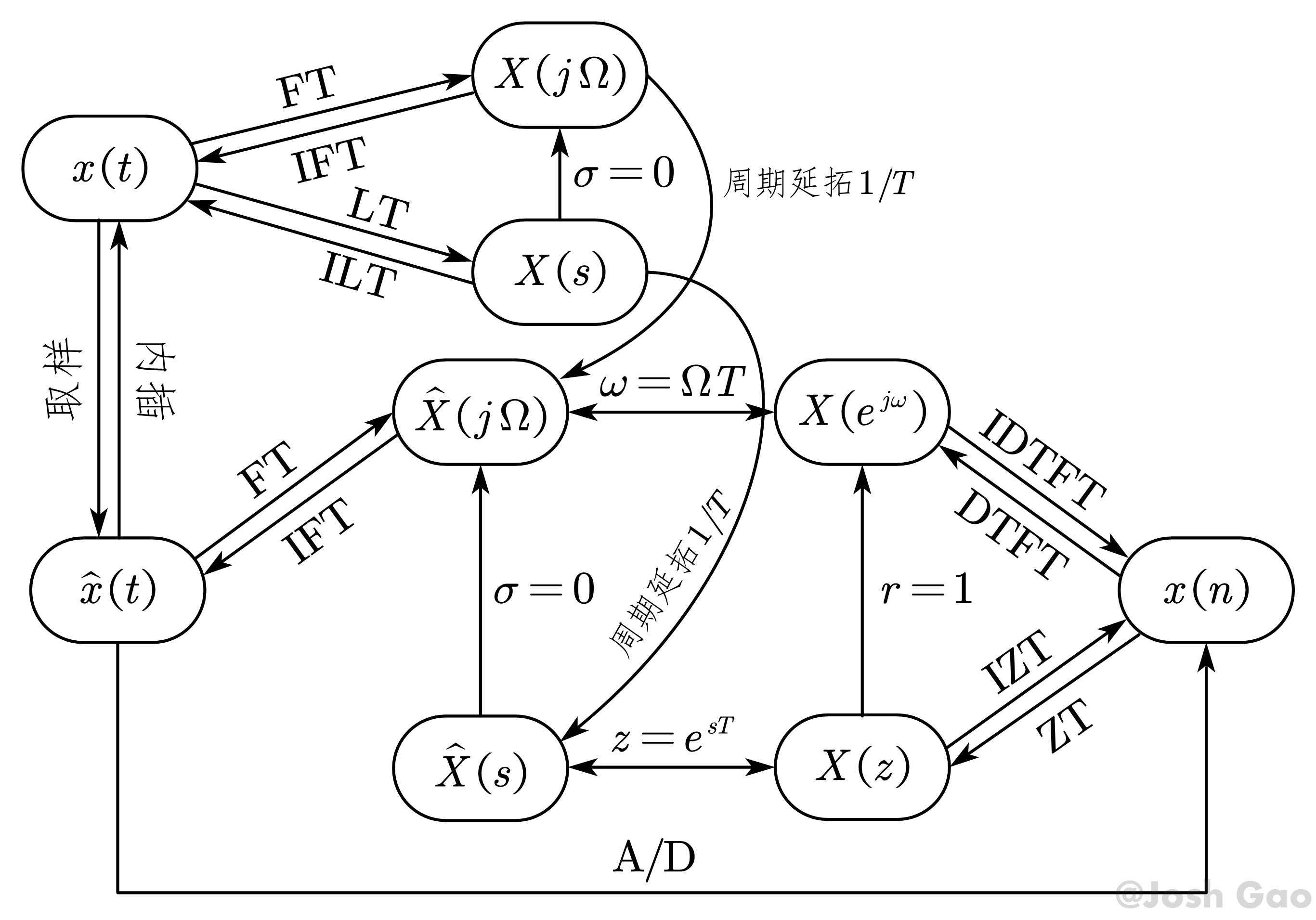+![傅里叶变换、拉氏变换和 $z$ 变换的关系](https://josh-blog-1257563604.cos.ap-beijing.myqcloud.com/img/2023-04-14-josh-dsp-part-1/2023-04-14-josh-dsp-part-1-010-RelationshipBetweenTransform.png?imageMogr2/thumbnail/!100p|watermark/2/text/QEpvc2ggR2Fv/font/YWhyb25iZC50dGY=/fontsize/80/dissolve/20/gravity/southeast/dx/5/dy/5){width=600px}
+
+# 参考文献
+
+王世一. *数字信号处理, 修订版.* 北京理工大学出版社, 1997.
+
+[^1]: $f\left( x \right)$ 的以 $2l$ 为周期的傅氏级数的指数形式为
+$$
+f\left(x\right)\sim\sum_{m=-\infty}^{\infty}{c_me^{jm\frac{x}{l}}}
+$$
+
+其中
+
+$$
+c_m=\frac{1}{2l}\int_{-l}^{l}{f\left(x\right)e^{-jm\frac{x}{l}}\mathrm{d}x}
+$$
+
+[^2]: 直接用 $p_\delta\left(t\right)$ 的傅里叶变换
+
+$$P_\delta\left(t\right)=\frac{2\pi}{T}\sum_{m=-\infty}^{\infty}{\delta(\Omega-m\Omega_s)}
+$$
+
+与 $x_a\left(t\right)$ 的傅里叶变换 $X_a\left(j\Omega\right)$ 卷积后除以 $2\pi$ 也可得到相应结果。
+
+[^3]: 即为周期方波的傅里叶变换。
+
+[^4]: 《信号与系统（第四版）》（曾禹村等编著，北京理工大学出版社，2018）中对 $\mathrm{sinc}$ 函数的定义不准确，严格来说归一化的 $\mathrm{sinc}$ 函数（常在信号处理领域应用）定义为 $\mathrm{sinc}\left(x\right)=\dfrac{\sin{\left(\pi x\right)}}{\pi x}$，而非归一化的 $\mathrm{sinc}$ 函数（常用在数学领域）定义为 $\mathrm{sinc}\left(x\right)=\dfrac{\sin{x}}{x}$。在信号处理中，为了区别归一化的 $\mathrm{sinc}$ 函数，定义取样函数（Sampling function）$\mathrm{Sa}\left(x\right)=\dfrac{\sin{x}}{x}$，但二者并无本质区别。
+
+[^5]: 时域卷积定理：$x\left(t\right)\ast y\left(t\right)=X\left(j\Omega\right)\cdot Y(j\Omega)$，频域卷积定理：$x\left(t\right)\cdot y\left(t\right)=\dfrac{1}{2\pi}X\left(j\Omega\right)\ast Y(j\Omega)$。

source/_posts/2023-04-14-josh-dsp-part-2.md

@@ -0,0 +1,251 @@
+---
+title: Josh 的学习笔记之数字信号处理（Part 2——离散傅里叶级数 DFS）
+mathjax: true
+comments: true
+copyright: true
+toc:
+  enable: true
+  number: false
+  wrap: true
+  expand_all: false
+  max_depth: 3
+tags:
+  - 数字信号和处理
+  - DSP
+  - 离散傅里叶级数
+  - DFS
+  - 连续时间傅里叶变换
+  - 连续傅里叶级数
+  - 离散时间傅里叶变换
+  - DTFT
+  - 圆周卷积
+  - 周期卷积
+  - 共轭对称
+categories:
+  - - Josh 的学习笔记
+    - 数字信号处理
+abbrlink: 3345523e
+date: 2023-04-14 18:43:17
+---
+
+# 1. 傅里叶变换的几种形式
+
+## 1.1 非周期连续时间信号的傅里叶变换
+
+  非周期连续时间信号的傅里叶变换（连续时间傅里叶变换，Continuous-Time Fourier Transform, CTFT）的形式为：
+
+$$\begin{equation}
+X_a\left(j\Omega\right)=\int_{-\infty}^{\infty}{x_a\left(t\right)e^{-j\Omega t}\mathrm{d}t}
+\end{equation}$$
+
+$$\begin{equation}
+x_a\left(t\right)=\frac{1}{2\pi}\int_{-\infty}^{\infty}{X_a\left(j\Omega\right)e^{j\Omega t}\mathrm{d}\Omega}
+\end{equation}$$
+
+<!-- more -->
+
+## 1.2 周期连续时间信号的傅里叶变换
+
+&emsp;&emsp;周期连续时间信号的傅里叶变换（连续傅里叶级数，Continous Fourier Series, CFS）的形式为：
+
+$$\begin{equation}
+X\left(m\Omega\right)=\frac{1}{t_p}\int_{-\frac{t_p}{2}}^{\frac{t_p}{2}}{x_a\left(t\right)e^{-jm\Omega t}\mathrm{d}t}
+\end{equation}$$
+
+$$\begin{equation}
+x_a\left(t\right)=\sum_{m=-\infty}^{\infty}{X\left(m\Omega\right)e^{jm\Omega t}}
+\end{equation}$$
+
+其中 $t_p$ 为信号的周期，频域相邻谱线间角频率增量 $\Omega=\dfrac{2\pi}{t_p}$。
+
+## 1.3 非周期离散时间信号的傅里叶变换
+
+&emsp;&emsp;非周期离散时间信号的傅里叶变换（离散时间傅里叶变换，Discrete-Time Fourier Transform, DTFT）的形式为：
+
+$$\begin{equation}
+X\left(e^{j\omega}\right)=\sum_{n=-\infty}^{\infty}{x\left(n\right)e^{-j\omega n}}
+\end{equation}$$
+
+$$\begin{equation}
+x\left(n\right)=\frac{1}{2\pi}\int_{-\pi}^{\pi}{X\left(e^{j\omega}\right)e^{j\omega n}\mathrm{d}\omega}
+\end{equation}$$
+
+取样频率 $f_s=\dfrac{1}{T}$，取样角频率 $\Omega_s=\dfrac{2\pi}{T}$，取样数字频率$\omega_s=2\pi$。
+
+## 1.4 周期离散时间信号的傅里叶变换
+
+&emsp;&emsp;周期离散时间信号的傅里叶变换（离散傅里叶级数，Discrete Fourier Series, DFS）的形式为：
+
+$$\begin{equation}
+\widetilde{X}\left(k\right)=\left.\widetilde{X}\left(e^{j\omega}\right)\right|_{\omega=k\frac{2\pi}{N}}=\sum_{n=0}^{N-1}{\widetilde{x}\left(n\right)e^{-j\frac{2\pi}{N}kn}}=\sum_{n=0}^{N-1}{\widetilde{x}\left(n\right)W_N^{kn}}
+\end{equation}$$
+
+$$\begin{equation}
+\widetilde{x}\left(n\right)=\frac{1}{N}\sum_{k=0}^{N-1}{\widetilde{X}\left(k\right)e^{j\frac{2\pi}{N}kn}}=\frac{1}{N}\sum_{k=0}^{N-1}{\widetilde{X}\left(k\right)W_N^{-kn}}
+\end{equation}$$
+
+其中 $N$ 为一个周期内的点数，时域相邻谱线间隔为 $T$ ，频域相邻谱线间隔为 $\dfrac{1}{NT}$，以数字频率表征时为 $\dfrac{2\pi}{N}$。
+
+> **由以上，在一个域中对函数进行取样，两取样点间增量的倒数，必是另一个域中的周期。**
+
+# 2. 离散傅里叶级数（DFS）的推导
+
+## 2.1 正变换
+
+&emsp;&emsp;令 $x\left(n\right)$ 为 $N$ 点长的离散序列，则其 DTFT（上标“~”用来表征周期性）
+
+$$\begin{equation}
+\widetilde{X}\left(e^{j\omega}\right)=\sum_{n=-\infty}^{\infty}{x\left(n\right)e^{-j\omega n}}=\sum_{n=0}^{N-1}{x\left(n\right)e^{-j\omega n}}
+\end{equation}$$
+
+对 $\widetilde{X}\left(e^{j\omega}\right)$ 取样，使其称为周期离散频率函数，由此时域序列 $x\left(n\right)$ 周期化为 $\widetilde{x}\left(n\right)$，令其谱线间隔为 $T$，则时域序列的周期为 $NT$，所以对频谱取样的谱间距为 $\dfrac{1}{NT}$，以数字频率表征时，谱间距
+
+$$\begin{equation}
+\omega_\mathrm{I}=\frac{2\pi}{N}
+\end{equation}$$
+
+因此，以数字频率 $\omega$ 为变量的 $X\left(e^{j\omega}\right)$ 被离散化时，其变量 $\omega$ 变为
+
+$$\begin{equation}
+\omega=k\omega_\mathrm{I}=k\frac{2\pi}{N}
+\end{equation}$$
+
+因此离散周期序列 $\widetilde{x}\left(n\right)$ 的傅里叶级数可写为
+
+$$\begin{equation}
+\widetilde{X}\left(k\right)=\left.\widetilde{X}\left(e^{j\omega}\right)\right|_{\omega=k\frac{2\pi}{N}}=\sum_{n=0}^{N-1}{\widetilde{x}\left(n\right)e^{-j\frac{2\pi}{N}kn}}=\sum_{n=0}^{N-1}{\widetilde{x}\left(n\right)W_N^{kn}}
+\end{equation}$$
+
+并将数字域频率用 $k$ 简化表示。且
+
+$$\begin{equation}
+\widetilde{X}\left(k+N\right)=\sum_{n=0}^{N-1}{\widetilde{x}\left(n\right)e^{-j\frac{2\pi}{N}\left(k+N\right)n}}=\sum_{n=0}^{N-1}{\widetilde{x}\left(n\right)e^{-j2\pi n}e^{-j\frac{2\pi}{N}kn}=}\sum_{n=0}^{N-1}{\widetilde{x}\left(n\right)e^{-j\frac{2\pi}{N}kn}=}\widetilde{X}\left(k\right)
+\end{equation}$$
+
+即 $\widetilde{X}\left(k\right)$ 是以 $N$ 为周期的周期函数。
+
+## 2.2 逆变换
+
+&emsp;&emsp;将正变换两边乘以 $e^{j\frac{2\pi}{N}kr}$，并在一个周期内求和，有
+
+$$\begin{equation}
+\sum_{k=0}^{N-1}{\widetilde{X}\left(k\right)e^{j\frac{2\pi}{N}kr}}=\sum_{k=0}^{N-1}{\left(\sum_{n=0}^{N-1}{\widetilde{x}\left(n\right)e^{-j\frac{2\pi}{N}kn}}\right)e^{j\frac{2\pi}{N}kr}}=N\left[\sum_{n=0}^{N-1}{\widetilde{x}\left(n\right)\left(\frac{1}{N}\sum_{k=0}^{N-1}e^{j\frac{2\pi}{N}k\left(r-n\right)}\right)}\right]
+\end{equation}$$
+
+由正交定理
+
+$$\begin{equation}
+\frac{1}{N}\sum_{k=0}^{N-1}e^{j\frac{2\pi}{N}k\left(r-n\right)}=
+\begin{aligned}
+\begin{cases}
+1,&r=n\\
+0,&r≠n
+\end{cases}
+\end{aligned}
+\end{equation}$$
+
+则
+
+$$\begin{equation}
+\sum_{k=0}^{N-1}{\widetilde{X}\left(k\right)e^{j\frac{2\pi}{N}kr}}=N\left.\left[\sum_{n=0}^{N-1}{\widetilde{x}\left(n\right)}\right]\right|_{n=r}=N\widetilde{x}\left(r\right)
+\end{equation}$$
+
+可得逆离散傅里叶变换
+
+$$\begin{equation}
+\widetilde{x}\left(n\right)=\frac{1}{N}\sum_{k=0}^{N-1}{\widetilde{X}\left(k\right)e^{j\frac{2\pi}{N}kn}}=\frac{1}{N}\sum_{k=0}^{N-1}{\widetilde{X}\left(k\right)W_N^{-kn}}
+\end{equation}$$
+
+且
+
+$$\begin{equation}
+\widetilde{x}\left(n+mN\right)=\frac{1}{N}\sum_{k=0}^{N-1}{\widetilde{X}\left(k\right)e^{j\frac{2\pi}{N}k\left(n+mN\right)}}=\frac{1}{N}\sum_{k=0}^{N-1}{\widetilde{X}\left(k\right)e^{j\frac{2\pi}{N}kn}e^{j2\pi km}}=\widetilde{x}\left(n\right)
+\end{equation}$$
+
+即 $\widetilde{x}\left(n\right)$ 是以 $N$ 为周期的周期函数。
+
+# 3. 离散傅里叶级数（DFS）的性质
+
+## 3.1 线性性质
+
+$$\begin{equation}
+\mathrm{DFS}\left[a{\widetilde{x}}_1\left(n\right)+{b\widetilde{x}}_2\left(n\right)\right]=a{\widetilde{X}}_1\left(k\right)+b{\widetilde{X}}_2\left(k\right)
+\end{equation}$$
+
+## 3.2 时移性质
+
+$$\begin{equation}
+\mathrm{DFS}\left[\widetilde{x}\left(n+m\right)\right]=W_N^{-mk}\widetilde{X}\left(k\right)
+\end{equation}$$
+
+证明：
+
+$$\begin{equation}
+\begin{aligned}
+\mathrm{DFS}\left[\widetilde{x}\left(n+m\right)\right]&=\sum_{n=0}^{N-1}{\widetilde{x}\left(n+m\right)W_N^{nk}}=\sum_{n=m}^{N-1+m}{\widetilde{x}\left(n\right)W_N^{\left(n-m\right)k}}=\sum_{n=m}^{N-1+m}{\widetilde{x}\left(n\right)W_N^{nk}W_N^{-mk}}
+\\
+&\xlongequal{利用\widetilde{x}\left(n\right)和W_N^{nk}的周期性}\left(\sum_{n=0}^{N-1}{\widetilde{x}\left(n\right)W_N^{nk}}\right)W_N^{-mk}=W_N^{-mk}\widetilde{X}\left(k\right)
+\end{aligned}
+\end{equation}$$
+
+## 3.3 频移性质
+
+$$\begin{equation}
+\mathrm{IDFS}\left[\widetilde{X}\left(k+l\right)\right]=W_N^{nl}\widetilde{x}\left(n\right)
+\end{equation}$$
+
+证明：
+
+$$\begin{equation}
+\begin{aligned}
+\mathrm{IDFS}\left[\widetilde{X}\left(k+l\right)\right]&=\frac{1}{N}\sum_{k=0}^{N-1}{\widetilde{X}\left(k+l\right)W_N^{-kn}}=\frac{1}{N}\sum_{k=l}^{N-1+l}{\widetilde{X}\left(k\right)W_N^{-\left(k-l\right)n}}=\frac{1}{N}\sum_{k=l}^{N-1+l}{\widetilde{X}\left(k\right)W_N^{-kn}W_N^{nl}}
+\\
+&\xlongequal{利用\widetilde{X}\left(n\right)和W_N^{-nk}的周期性}\frac{1}{N}\left(\sum_{k=0}^{N-1}{\widetilde{X}\left(k\right)W_N^{-kn}}\right)W_N^{nl}=W_N^{nl}\widetilde{x}\left(n\right)
+\end{aligned}
+\end{equation}$$
+
+## 3.4 时域周期卷积
+
+$$\begin{equation}
+{\widetilde{x}}_1\left(n\right)\odot{\widetilde{x}}_2\left(n\right)=\mathrm{IDFS}\left[{\widetilde{X}}_1\left(k\right)\cdot{\widetilde{X}}_2\left(k\right)\right]
+\end{equation}$$
+
+证明：
+
+$$\begin{equation}
+\begin{aligned}
+\mathrm{IDFS}\left[{\widetilde{X}}_1\left(k\right)\cdot{\widetilde{X}}_2\left(k\right)\right]&=\frac{1}{N}\sum_{k=0}^{N-1}{\left[{\widetilde{X}}_1\left(k\right)\cdot{\widetilde{X}}_2\left(k\right)\right]W_N^{-nk}}\\
+&=\frac{1}{N}\sum_{k=0}^{N-1}{\left[\sum_{m=0}^{N-1}{\widetilde{x}}_1\left(m\right)W_N^{mk}\right]{\widetilde{X}}_2\left(k\right)W_N^{-nk}}\\
+&=\frac{1}{N}\sum_{k=0}^{N-1}\left[\sum_{m=0}^{N-1}{\widetilde{x}}_1\left(m\right){\widetilde{X}_2\left(k\right)W}_N^{-\left(n-m\right)k}\right]\\
+&=\sum_{m=0}^{N-1}{\widetilde{x}}_1\left(m\right)\left[\frac{1}{N}\sum_{k=0}^{N-1}{\widetilde{X}_2\left(k\right)W}_N^{-\left(n-m\right)k}\right]\\
+&=\sum_{m=0}^{N-1}{\widetilde{x}}_1\left(m\right){\widetilde{x}}_2\left(n-m\right)
+\\
+&={\widetilde{x}}_1\left(n\right)\odot{\widetilde{x}}_2\left(n\right)
+\end{aligned}
+\end{equation}$$
+
+> 注：此处用 $\odot$ 表示圆周卷积，不同教材中圆周卷积的符号表述可能不同。
+
+## 3.5 频域周期卷积
+
+$$\begin{equation}
+\mathrm{DFS}\left[{\widetilde{x}}_1\left(n\right){\widetilde{x}}_2\left(n\right)\right]=\frac{1}{N}\left[{\widetilde{X}}_1\left(k\right)\odot{\widetilde{X}}_2\left(k\right)\right]
+\end{equation}$$
+
+证明：
+
+$$\begin{equation}
+\begin{aligned}
+\mathrm{DFS}\left[{\widetilde{x}}_1\left(n\right){\widetilde{x}}_2\left(n\right)\right]&=\sum_{n=0}^{N-1}{\widetilde{X}_1\left(n\right){\widetilde{x}}_2\left(n\right)W_N^{kn}}=\sum_{n=0}^{N-1}\left[\frac{1}{N}\sum_{r=0}^{N-1}{\widetilde{X}_1\left(r\right)W_N^{-rn}}\right]{\widetilde{x}}_2\left(n\right)W_N^{kn}\\
+&=\frac{1}{N}\sum_{n=0}^{N-1}\left[\sum_{r=0}^{N-1}{\widetilde{X}_1\left(r\right){\widetilde{x}}_2\left(n\right)W_N^{\left(k-r\right)n}}\right]\\
+&=\frac{1}{N}\sum_{r=0}^{N-1}{\widetilde{X}}_1\left(r\right)\left[\sum_{k=0}^{N-1}{\widetilde{X}_2\left(n\right)W_N^{\left(k-r\right)n}}\right]\\
+&=\frac{1}{N}\sum_{r=0}^{N-1}{\widetilde{X}}_1\left(r\right){\widetilde{X}}_2\left(k-r\right)\\
+&=\frac{1}{N}\left[{\widetilde{X}}_1\left(k\right)\odot{\widetilde{X}}_2\left(k\right)\right]
+\end{aligned}
+\end{equation}$$
+
+> 注：此处用 $\odot$ 表示圆周卷积，不同教材中圆周卷积的符号表述可能不同。
+
+# 参考文献
+
+王世一. *数字信号处理, 修订版.* 北京理工大学出版社, 1997.

source/_posts/2023-04-14-josh-dsp-part-3.md

@@ -0,0 +1,564 @@
+---
+title: Josh 的学习笔记之数字信号处理（Part 3——离散傅里叶变换 DFT）
+mathjax: true
+comments: true
+copyright: true
+toc:
+  enable: true
+  number: false
+  wrap: true
+  expand_all: false
+  max_depth: 4
+abbrlink: fd9f9a29
+date: 2023-04-14 22:17:40
+tags:
+  - 数字信号和处理
+  - DSP
+  - 离散傅里叶变换
+  - DFT
+  - 延长序列
+  - 圆周卷积
+  - 重叠相加
+  - 重叠保留
+  - 内插公式
+  - 混叠
+  - 频谱泄露
+  - 栅栏效应
+categories:
+  - - Josh 的学习笔记
+    - 数字信号处理
+---
+
+# 1. 离散傅里叶变换（Discrete Fourier Transform, DFT）的定义
+
+  取离散傅里叶级数的主值，得离散傅里叶变换
+
+$$\begin{equation}
+X\left(k\right)=\widetilde{X}\left(k\right)R_N\left(k\right)=\sum_{n=0}^{N-1}{x\left(n\right)W_N^{kn}},\ \ k=0,1,\cdots,N-1
+\end{equation}$$
+
+$$\begin{equation}
+x\left(n\right)=\widetilde{x}\left(n\right)R_N\left(n\right)=\frac{1}{N}\sum_{k=0}^{N-1}{X\left(k\right)W_N^{-kn}},\ \ n=0,1,\cdots,N-1
+\end{equation}$$
+
+且 $\widetilde{X}\left(k\right)=X\left(\left(k\right)\right)_N,\widetilde{x}\left(n\right)=x\left(\left(n\right)\right)_N$。其中 $R_N\left(n\right)$ 表示矩形序列，表示取主值；$\left(\left(n\right)\right)_N$ 表示 $n$ 对 $N$ 取余。
+
+> 注：不同教材中取主值、取余的符号表述可能不同。
+
+<!-- more -->
+
+# 2. DFT 的矩阵算法
+
+&emsp;&emsp;若令 $X=\left[\begin{matrix}X\left(0\right)&X\left(1\right)&\cdots&X\left(N-1\right)\\\end{matrix}\right]^\mathrm{T}，x=\left[\begin{matrix}x\left(0\right)&x\left(1\right)&\cdots&x\left(N-1\right)\\\end{matrix}\right]^\mathrm{T}$，则 DFT 和 IDFT 可分别表示为
+
+$$\begin{equation}
+X=D_Nx,\ \ x=D_N^{-1}X
+\end{equation}$$
+
+其中 Vandermonde 矩阵
+
+$$\begin{equation}
+D_N=\left[\begin{matrix}1&1&1&\cdots&1\\1&W_N^1&W_N^2&\cdots&W_N^{\left(N-1\right)}\\1&W_N^2&W_N^4&\cdots&W_N^{2\left(N-1\right)}\\\vdots&\vdots&\vdots&&\vdots\\1&W_N^{\left(N-1\right)}&W_N^{2\left(N-1\right)}&\cdots&W_N^{\left(N-1\right)^2}\\\end{matrix}\right]
+\end{equation}$$
+
+$$\begin{equation}
+D_N^{-1}=\frac{1}{N}\left[\begin{matrix}1&1&1&\cdots&1\\1&W_N^{-1}&W_N^{-2}&\cdots&W_N^{-\left(N-1\right)}\\1&W_N^{-2}&W_N^{-4}&\cdots&W_N^{-2\left(N-1\right)}\\\vdots&\vdots&\vdots&&\vdots\\1&W_N^{-\left(N-1\right)}&W_N^{-2\left(N-1\right)}&\cdots&W_N^{-\left(N-1\right)^2}\\\end{matrix}\right]
+\end{equation}$$
+
+且有 $D_N^{-1}=\dfrac{1}{N}D_N^\ast$。
+
+# 3. 离散傅里叶变换（DFT）的性质
+
+## 3.1 线性性质
+
+$$\begin{equation}
+\mathrm{DFT}\left[ax_1\left(n\right)+{bx}_2\left(n\right)\right]=aX_1\left(k\right)+bX_2\left(k\right)
+\end{equation}$$
+
+## 3.2 用正变换计算逆变换
+
+$$\begin{equation}
+x\left(n\right)=\frac{1}{N}\left[\sum_{k=0}^{N-1}{X^\ast\left(k\right)W_N^{nk}}\right]^\ast,\ \ n=0,1,\cdots,N-1
+\end{equation}$$
+
+证明：
+
+$$\begin{equation}
+\frac{1}{N}\left[\sum_{k=0}^{N-1}{X^\ast\left(k\right)W_N^{nk}}\right]^\ast=\frac{1}{N}\left[\sum_{k=0}^{N-1}{X\left(k\right)W_N^{-nk}}\right]=x\left(n\right)
+\end{equation}$$
+
+## 3.3 对称定理
+
+$$\begin{equation}
+\mathrm{DFT}\left[\frac{1}{N}X\left(n\right)\right]=x\left(-k\right)=x\left(N-k\right)
+\end{equation}$$
+
+证明：
+
+$$\begin{equation}
+\begin{aligned}
+&x\left(-n\right)=x\left(N-n\right)=\frac{1}{N}\sum_{k=0}^{N-1}{X\left(k\right)W_N^{-\left(N-n\right)k}}=\frac{1}{N}\sum_{k=0}^{N-1}{X\left(k\right)W_N^{nk}}
+\\
+\Longrightarrow &x\left(-k\right)=x\left(N-k\right)=\sum_{n=0}^{N-1}{\left[\frac{X\left(n\right)}{N}\right]W_N^{kn}}=\mathrm{DFT}\left[\frac{X\left(n\right)}{N}\right]
+\end{aligned}
+\end{equation}$$
+
+## 3.4 反转定理
+
+$$\begin{equation}
+\mathrm{DFT}\left[x\left(-n\right)\right]=X\left(-k\right)
+\end{equation}$$
+
+证明：
+
+$$\begin{equation}
+\mathrm{DFT}\left[x\left(-n\right)\right]=\sum_{n=0}^{N-1}{x\left(-n\right)W_N^{nk}}\xlongequal{令m=-n}\sum_{m=-\left(N-1\right)}^{0}{x\left(m\right)W_N^{-mk}}=\sum_{m=0}^{N-1}{x\left(m\right)W_N^{m\cdot\left(-k\right)}}=X\left(-k\right)
+\end{equation}$$
+
+## 3.5 序列的总和
+
+$$\begin{equation}
+\sum_{n=0}^{N-1}x\left(n\right)=\left.\sum_{n=0}^{N-1}{x\left(n\right)W_N^{kn}}\right|_{k=0}\left.=X\left(k\right)\right|_{k=0}=X\left(0\right)
+\end{equation}$$
+
+## 3.6 序列的起始值
+
+$$\begin{equation}
+x\left(0\right)=\frac{1}{N}\left.\sum_{k=0}^{N-1}{X\left(k\right)W_N^{-kn}}\right|_{n=0}=\frac{1}{N}\sum_{k=0}^{N-1}X\left(k\right)
+\end{equation}$$
+
+## 3.7 延长序列的 DFT
+
+&emsp;&emsp;将 $N$ 点长序列 $x\left(n\right)\left(n=1,2,\cdots,N-1\right)$ 补零延长 $rN$ 点得到序列 $g\left(n\right)$，即
+
+$$\begin{equation}
+g\left(n\right)=
+\begin{aligned}
+\begin{cases}
+x(n),&n=0,1,⋯,N-1\\
+0,&n=N,N+1,⋯rN-1
+\end{cases}
+\end{aligned}
+\end{equation}$$
+
+则 $g\left(n\right)$ 的 DFT
+
+$$\begin{equation}
+\begin{aligned}
+G\left(k\right)&=\mathrm{DFT}\left[g\left(n\right)\right]=\sum_{n=0}^{rN-1}{g\left(n\right)e^{-j\frac{2\pi nk}{rN}}}=\sum_{n=0}^{N-1}{g\left(n\right)e^{-j\frac{2\pi n\left(\frac{k}{r}\right)}{N}}}
+\\
+&=X\left(\frac{k}{r}\right),\ \ k=0,1,\cdots,rN-1\
+\end{aligned}
+\end{equation}$$
+
+由此，**$G\left(k\right)$ 与 $X\left(k\right )$具有相同的形状，但 $G\left(k\right)$ 的频谱间隔比 $X\left(k\right)$ 的小。即 {% label primary @通过补零，频谱变得更加细致。但是补零不能提高频谱分辨能力。%}**
+
+## 3.8 有限长序列的圆周特性
+
+### 3.8.1 圆周移位（周期化→移位→取主值）
+
+$$\begin{equation}
+x\left(\left(n-m\right)\right)_NR_N\left(n\right)=
+\begin{aligned}
+\begin{cases}
+x\left(n-m\right),&m\leqslant n\leqslant N-1
+\\
+x\left(N-m+n\right),&0\leqslant n\leqslant m
+\end{cases}
+\end{aligned}
+\end{equation}$$
+
+### 3.8.2 圆周反转（周期化→反转→取主值）
+
+$$\begin{equation}
+x\left(\left(-n\right)\right)_NR_N\left(n\right)=
+\begin{aligned}
+\begin{cases}
+x\left(0\right),&n=0
+\\
+x\left(N-n\right),&1\leqslant n\leqslant N-1
+\end{cases}
+\end{aligned}
+\end{equation}$$
+
+### 3.8.3 有限长序列的时间圆周移位定理（可以通过 DFS 证明）
+
+$$\begin{equation}
+\mathrm{DFT}\left[x\left(\left(n+m\right)\right)_NR_N\left(n\right)\right]=W_N^{-mk}X\left(k\right)
+\end{equation}$$
+
+由此，**有限长序列的圆周移位导致频谱线性相移，而对频谱幅度无影响**。
+
+### 3.8.4 限长序列的频率圆周移位定理（调制特性，可以通过 DFS 证明）
+
+$$\begin{equation}
+\mathrm{IDFT}\left[X\left(\left(k+l\right)\right)_NR_N\left(k\right)\right]=W_N^{nl}x\left(n\right)=e^{-j\frac{2\pi}{N}nl}x\left(n\right)
+\end{equation}$$
+
+由此，**时域序列的调制等效于频域的圆周移位**，且可以推得
+
+$$\begin{equation}
+\mathrm{DFT}\left[x\left(n\right)\cos{\left(\frac{2\pi nl}{N}\right)}\right]=\frac{1}{2}\left[X\left(\left(k-l\right)\right)_N+X\left(\left(k+l\right)\right)_N\right]R_N\left(k\right)
+\end{equation}$$
+
+$$\begin{equation}
+\mathrm{DFT}\left[x\left(n\right)\sin{\left(\frac{2\pi nl}{N}\right)}\right]=\frac{1}{2}\left[X\left(\left(k-l\right)\right)_N-X\left(\left(k+l\right)\right)_N\right]R_N\left(k\right)
+\end{equation}$$
+
+### 3.8.5 DFT的圆周对称性
+
+#### 3.8.5.1 奇序列和偶序列的 DFT
+
+奇序列的 DFT
+
+$$\begin{equation}
+x\left(n\right)=-x\left(-n\right)=-x\left(\left(-n\right)\right)_NR_N\left(n\right)\rightarrow X\left(k\right)=-X\left(-k\right)=-X\left(\left(N-k\right)\right)_NR_N\left(k\right)
+\end{equation}$$
+
+偶序列的 DFT
+
+$$\begin{equation}
+x\left(n\right)=x\left(-n\right)=x\left(\left(-n\right)\right)_NR_N\left(n\right)\rightarrow X\left(k\right)=X\left(-k\right)=X\left(\left(N-k\right)\right)_NR_N\left(k\right)
+\end{equation}$$
+
+#### 3.8.5.2 序列的对称分解
+
+&emsp;&emsp;普通序列 $x\left(n\right)$ 的共轭对称分量和共轭反对称分量分别为
+
+$$\begin{equation}
+x_e\left(n\right)=\frac{1}{2}\left[x\left(n\right)+x^\ast\left(-n\right)\right],\ \ x_o\left(n\right)=\frac{1}{2}\left[x\left(n\right)-x^\ast\left(-n\right)\right]
+\end{equation}$$
+
+对有限长序列的 DFT 进行分析时，定义周期共轭对称分量和周期共轭反对称分量分别为
+
+$$\begin{equation}
+x_{ep}\left(n\right)=\frac{1}{2}\left[x\left(\left(n\right)\right)_N+x^\ast\left(\left(-n\right)\right)_N\right]R_N\left(n\right)=\frac{1}{2}\left[x\left(n\right)+x^\ast\left(N-n\right)\right]
+\end{equation}$$
+
+$$\begin{equation}
+x_{op}\left(n\right)=\frac{1}{2}\left[x\left(\left(n\right)\right)_N-x^\ast\left(\left(-n\right)\right)_N\right]R_N\left(n\right)=\frac{1}{2}\left[x\left(n\right)-x^\ast\left(N-n\right)\right]
+\end{equation}$$
+
+二者关系为
+
+$$\begin{equation}
+x_{ep}\left(n\right)=\left[x_e\left(n\right)+x_e\left(n-N\right)\right]R_N\left(n\right),\ \ x_{op}\left(n\right)=\left[x_o\left(n\right)+x_o\left(n-N\right)\right]R_N\left(n\right)
+\end{equation}$$
+
+<a id=3.8.5.3></a>
+
+#### 3.8.5.3 共轭复序列的 DFT
+
+$$\begin{equation}
+\mathrm{DFT}\left[x^\ast\left(n\right)\right]=X^\ast\left(\left(N-k\right)\right)_N
+\end{equation}$$
+
+$$\begin{equation}
+\mathrm{DFT}\left[x^\ast\left(-n\right)\right]=X^\ast\left(k\right)
+\end{equation}$$
+
+证明：
+
+$$\begin{equation}
+\mathrm{DFT}\left[x^\ast\left(n\right)\right]=\sum_{n=0}^{N-1}{x^\ast\left(n\right)W_N^{kn}}=\left[\sum_{n=0}^{N-1}{x\left(n\right)W_N^{-kn}}\right]^\ast=X^\ast\left(-k\right)=X^\ast\left(\left(N-k\right)\right)_N
+\end{equation}$$
+
+$$\begin{equation}
+\begin{aligned}
+\mathrm{DFT}\left[x^\ast\left(-n\right)\right]&=\sum_{n=0}^{N-1}{x^\ast\left(-n\right)W_N^{kn}}=\left[\sum_{n=0}^{N-1}{x\left(-n\right)W_N^{-kn}}\right]^\ast
+\\
+&=\left[\sum_{m=-N+1}^{0}{x\left(m\right)W_N^{km}}\right]^\ast=\left[\sum_{n=0}^{N-1}{x\left(n\right)W_N^{kn}}\right]^\ast=X^\ast\left(k\right)
+\end{aligned}
+\end{equation}$$
+
+<a id=3.8.5.4></a>
+
+#### 3.8.5.4 复数序列的 DFT
+
+$$\begin{equation}
+x\left(n\right)=x_r\left(n\right)+jx_i\left(n\right)
+\end{equation}$$
+
+$$\begin{equation}
+\quad\quad\quad\updownarrow\qquad\quad \updownarrow
+\end{equation}$$
+
+$$\begin{equation}
+X\left(k\right)=X_{ep}\left(k\right)+X_{op}\left(k\right)
+\end{equation}$$
+
+证明：
+
+$$\begin{equation}
+X_{ep}\left(k\right)=\mathrm{DFT}\left[x_r\left(n\right)\right]=\frac{1}{2}\mathrm{DFT}\left[x\left(n\right)+x^\ast\left(n\right)\right]=\frac{1}{2}\left[X\left(k\right)+X^\ast\left(N-k\right)\right]
+\end{equation}$$
+
+$$\begin{equation}
+X_{op}\left(k\right)=\mathrm{DFT}\left[{jx}_i\left(n\right)\right]=\frac{1}{2}\mathrm{DFT}\left[x\left(n\right)-x^\ast\left(n\right)\right]=\frac{1}{2}\left[X\left(k\right)+X^\ast\left(N-k\right)\right]
+\end{equation}$$
+
+且由 [3.8.5.3 共轭复序列的 DFT](#3.8.5.3) 可推知
+
+$$\begin{equation}
+X_{ep}\left(k\right)=X_{ep}^\ast\left(N-k\right)\ \ \ (实部相等，虚部相反)
+\end{equation}$$
+
+$$\begin{equation}
+X_{op}\left(k\right)=-X_{op}^\ast\left(N-k\right)(实部相反，虚部相等)
+\end{equation}$$
+
+#### 3.8.5.5 DFT 的奇偶虚实特性
+
+| $x(n)$ |       $X(k)$       |
+| :----: | :----------------: |
+|   偶   |         偶         |
+|   奇   |         奇         |
+|   实   | 实部为偶，虚部为奇 |
+|   虚   | 实部为奇，虚部为偶 |
+|  实偶  |        实偶        |
+|  实奇  |        虚奇        |
+|  虚偶  |        虚偶        |
+|  虚奇  |        实奇        |
+
+### 3.8.6 圆周卷积定理
+
+> 注：此处用 $\odot$ 表示圆周卷积，不同教材中圆周卷积的符号表述可能不同。
+
+#### 3.8.6.1 时域圆周卷积定理
+
+$$\begin{equation}
+\begin{aligned}
+x\left(n\right)=x_1\left(n\right)\odot x_2\left(n\right)&=\widetilde{y}\left(n\right)=\sum_{m=0}^{N-1}{x_1\left(m\right)\left[x_2\left(\left(n-m\right)\right)_NR_N\left(n\right)\right]}
+\\
+&=\mathrm{IDFT}\left[X_1\left(k\right)\cdot X_2\left(k\right)\right]
+\end{aligned}
+\end{equation}$$
+
+#### 3.8.6.2 频域圆周卷积定理
+
+$$\begin{equation}
+\begin{aligned}
+X\left(k\right)=X_1\left(k\right)\odot X_2\left(k\right)&=\widetilde{X}\left(k\right)R_N\left(k\right)=\frac{1}{N}\sum_{l=0}^{N-1}{X_1\left(l\right)\left[X_2\left(\left(k-l\right)\right)_NR_N\left(k\right)\right]}
+\\
+&=\mathrm{DFT}\left[x_1\left(n\right)\cdot x_2\left(n\right)\right]
+\end{aligned}
+\end{equation}$$
+
+#### 3.8.6.3 圆周卷积和线性卷积的关系
+
+&emsp;&emsp;长度为 $L$ 的序列 $x_1\left(n\right)$ 和长度为 $M$ 的序列 $x_2\left(n\right)$ 的周期卷积是二者的线性卷积的以 $N$ 为周期的周期延拓，若满足
+
+$$\begin{equation}
+N\geqslant L+M-1
+\end{equation}$$
+
+则周期卷积的主值序列即圆周卷积与线性卷积完全相同，即 $x_1\left(n\right)\odot x_2\left(n\right)=x_1\left(n\right)\ast x_2\left(n\right)$
+
+#### 3.8.6.4 圆周卷积的矩阵算法
+
+$$\begin{equation}
+y=h\odot x=\left[\begin{matrix}h_1&0&\cdots&0&h_m&\cdots\\h_2&h_1&\cdots&0&0&\cdots\\\vdots&\vdots&&\vdots&\vdots&\cdots\\h_m&h_{m-1}&\cdots&0&0&\cdots\\0&h_m&\cdots&h_1&0&\cdots\\0&0&&\vdots&h_1&\cdots\\\vdots&\vdots&&h_{m-1}&\vdots&\cdots\\0&0&\cdots&h_m&h_{m-1}&\cdots\\\end{matrix}\right]_{N\times N}\cdot\left[\begin{matrix}x_1\\x_2\\\vdots\\x_n\\0\\\vdots\\0\\\end{matrix}\right]_{N\times1}
+\end{equation}$$
+
+也可先计算线性卷积以 $N$ 为周期进行周期化后取主值得到圆周卷积。注意周期化时 $N<m+n-1$ 的情况，此时会出现重叠，重叠部分相加后才是圆周卷积的结果。
+
+### 3.8.7 重叠相加法和重叠保留法
+
+**例**&emsp;已知序列
+
+$$\begin{equation}x\left(n\right)=\left\{2,-3,4,5,-6,7,8,-9,-10,11,-12,-13,-14\right\}\left(0\leqslant n\leqslant12\right)
+\end{equation}$$
+
+$$\begin{equation}
+h\left(n\right)=\left\{1,-2,-3\right\}(0\leqslant n\leqslant2)
+\end{equation}$$
+
+&emsp;&emsp;试分别用重叠相加法和重叠保留法计算线性卷积，取分段长度 $L=5$。
+
+解：①重叠相加法
+
+&emsp;&emsp;&emsp;将长序列 $x\left(n\right)$ 分段，每段长度为 $5$
+
+$$\begin{equation}
+\begin{aligned}
+&x_1\left(n\right)=\left\{2,-3,4,5,-6\right\} \\
+&x_2\left(n\right)=\left\{7,8,-9,-10,11\right\} \\
+&x_3\left(n\right)=\left\{ -12,-13,-14\right\}
+\end{aligned}
+\end{equation}$$
+
+&emsp;&emsp;&emsp;用圆周卷积计算计算各段与 $h\left(n\right)$ 的线性卷积，下划线标注部分是需要重叠相加的部分
+
+$$\begin{equation}
+\begin{aligned}
+&y_1\left(n\right)=\left\{2,-7,4,6,-28,\underline{-3,18}\right\}\\
+&y_2\left(n\right)=\left\{\underline{7,-6},-46,-16,58,\underline{8,-33}\right\}\\
+&y_3\left(n\right)=\left\{\underline{-12,11},48,67,42\right\}
+\end{aligned}
+\end{equation}$$
+
+&emsp;&emsp;&emsp;将各段结果重叠相加，连接成线性卷积结果
+
+$$\begin{equation}
+y\left(n\right)=\left\{2,-7,4,6,-28,\mathbf{4},\mathbf{12},-46,-16,58,-\mathbf{4},-\mathbf{22},48,67,42\right\}
+\end{equation}$$
+
+&emsp;&emsp;②重叠保留法
+
+&emsp;&emsp;&emsp;将长序列 $x\left(n\right)$ 分段，每段长度为 $5$
+
+$$\begin{equation}
+\begin{aligned}
+&x_1\left(n\right)=\left\{\underline{0,0,2},-3,4\right\}\\
+&x_2\left(n\right)=\left\{\underline{-3,4},5,-6,7\right\}\\
+&x_3\left(n\right)=\left\{\underline{-6,-7},8,-9,-10\right\}\\
+&x_4\left(n\right)=\left\{\underline{-9,-10},11,-12,-13\right\}\\
+&x_5\left(n\right)=\left\{\underline{-12,-13},-14,0,0\right\}
+\end{aligned}
+\end{equation}$$
+
+&emsp;&emsp;&emsp;用圆周卷积计算计算各段与 $h\left(n\right)$ 的线性卷积，下划线标注部分是需要舍去的部分
+
+$$\begin{equation}
+\begin{aligned}
+&y_1\left(n\right)=\left\{\underline{1,-12},2,-7,4\right\}\\
+&y_2\left(n\right)=\left\{\underline{1,-11},6,28,4\right\}\\
+&y_3\left(n\right)=\left\{\underline{41,49},12,-46,-16\right\}\\
+&y_4\left(n\right)=\left\{\underline{53,47},58,-4,-22\right\}\\
+&y_5\left(n\right)=\left\{\underline{-12,11},48,67,42\right\}
+\end{aligned}
+\end{equation}$$
+
+&emsp;&emsp;&emsp;将各段重叠部分舍去，连接成线性卷积结果
+
+$$\begin{equation}
+y\left(n\right)=\left\{2,-7,4,6,-28,4,12,-46,-16,58,-4,-22,48,67,42\right\}
+\end{equation}$$
+
+## 3.9 Parseval 定理（能量守恒）
+
+$$\begin{equation}
+\sum_{n=0\ }^{N-1}{x^2\left(n\right)}=\frac{1}{N}\sum_{k=0}^{N-1}\left|X\left(k\right)\right|^2
+\end{equation}$$
+
+## 3.10 DFT 与 $z$ 变换
+
+$$\begin{equation}
+\begin{aligned}
+X\left(k\right)&=\sum_{n=0}^{N-1}{x\left(n\right)W_N^{nk}}=\sum_{n=0}^{N-1}{x\left(n\right)e^{-j\frac{2\pi}{N}nk}}=\left.\sum_{n=0}^{N-1}{x\left(n\right)z^{-n}}\right|_{z=e^{j\frac{2\pi}{N}k}}
+\\
+&=\left.X\left(z\right)\right|_{z=e^{j\frac{2\pi}{N}k}}=\left.\sum_{n=0}^{N-1}{x\left(n\right)e^{-j\omega n}}\right|_{\omega=\frac{2\pi}{N}k}\left(k=0,1,\cdots,N-1\right)
+\end{aligned}
+\end{equation}$$
+
+因此 $x\left(n\right)$ 的 DFT 的 $N$ 个系数即为 $x\left(n\right)$ 的 $z$ 变换 $X\left(z\right)$ 在单位圆上 $N$ 等分的取样点。
+
+# 4. 频域取样的点数限制
+
+&emsp;&emsp;设 $M$ 点序列 $x\left(n\right)$ 的 $z$ 变换为 $X\left(z\right)$，DTFT 为 $X\left(e^{j\omega}\right)$，则有
+
+> 在 $X\left(z\right)$ 的单位圆上均匀采样 $N$ 点，其 IDFT 是序列 $x\left(n\right)$ 以周期 $N$ 进行周期延拓后的主值序列；
+>
+> 在 $X\left(e^{j\omega}\right)$ 的一个周期内均匀采样 $N$ 点，其 IDFT 是序列 $x\left(n\right)$ 以周期 $N$ 进行周期延拓后的主值序列；
+>
+> 在 $X\left(e^{j\omega}\right)$ 的一个周期内均匀采样 $M$ 点，其 IDFT 是序列 $x\left(n\right)$ 本身。
+
+由此，对于列长为M的有限长序列 $x\left(n\right)$，频域取样不失真的条件是取样点数 $N$ 满足
+
+$$\begin{equation}
+N\geqslant M
+\end{equation}$$
+
+并且对于无限长序列 $x\left(n\right)$，无论 $N$ 取值如何，都不可能消除混叠，只能随着取样点 $N$ 增加而接近 $x\left(n\right)$。
+
+# 5. 内插公式
+
+&emsp;&emsp;用 DFT 表示 ZT
+
+$$\begin{equation}
+\begin{aligned}
+X\left(z\right)&=\sum_{n=0}^{N-1}{x\left(n\right)z^{-n}}=\sum_{n=0}^{N-1}{\left[\frac{1}{N}\sum_{k=0}^{N-1}{X\left(k\right)W_N^{-nk}}\right]z^{-n}}=\frac{1}{N}\sum_{k=0}^{N-1}\left[X\left(k\right)\sum_{n=0}^{N-1}\left(W_N^{-k}z^{-1}\right)^n\right]
+\\
+&=\frac{1}{N}\sum_{k=0}^{N-1}{X\left(k\right)\frac{1-W_N^{-kn}z^{-N}}{1-W_N^{-k}z^{-1}}}=\frac{1}{N}\sum_{k=0}^{N-1}{X\left(k\right)\frac{1-z^{-N}}{1-W_N^{-k}z^{-1}}}
+\\
+&=\frac{1-z^{-N}}{N}\sum_{k=0}^{N-1}\frac{X\left(k\right)}{1-W_N^{-k}z^{-1}}=\sum_{k=0}^{N-1}{X\left(k\right)\varphi_k\left(z\right)}
+\end{aligned}
+\end{equation}$$
+
+其中 $X\left(z\right)$ 的内插公式
+
+$$\begin{equation}
+\varphi_k\left(z\right)=\frac{1}{N}\cdot\frac{1-z^{-N}}{1-W_N^{-k}z^{-1}}
+\end{equation}$$
+
+&emsp;&emsp;用 DFT 表示 DTFT
+
+$$\begin{equation}
+X\left(e^{j\omega}\right)=\left.X\left(z\right)\right|_{z=e^{j\omega}}=\sum_{k=0}^{N-1}{X\left(k\right)\varphi_k\left(e^{j\omega}\right)}=\sum_{k=0}^{N-1}X\left(k\right)\varphi\left(\omega-k\frac{2\pi}{N}\right)
+\end{equation}$$
+
+其中内插函数
+
+$$\begin{equation}
+\varphi\left(\omega\right)=\frac{1}{N}\frac{\sin{\left(\frac{\omega N}{2}\right)}}{\sin{\left(\frac{\omega}{2}\right)}}e^{-j\omega\left(\frac{N-1}{2}\right)}
+\end{equation}$$
+
+**时域取样定理说明，对频域带限的信号，可对其进行时域取样而不丢失任何信息。频域取样理论说明，时间有限的信号（有限长序列），也可对其进行频域取样（DFT）而不丢失任何信息。**
+
+# 6. 用 DFT 对连续时间信号逼近的问题
+
+## 6.1 混叠现象
+
+&emsp;&emsp;时域采样会引起频谱周期化，通过 $f_s\geqslant 2f_h$ 消除。
+
+## 6.2 频谱泄露现象
+
+&emsp;&emsp;取用有限个数据，即将信号截断的过程，等同于将信号乘以窗函数。如果窗函数是矩形窗，在时域内将信号截断相当于乘以矩形窗，而在频域中则相当于原信号的频谱与矩形窗的频谱卷积，使得原信号的频谱被展宽，造成频谱泄露。**通常通过选择频谱特性更接近于 $\delta\left(k\right)$ 的函数来减少频谱泄露。**
+
+## 6.3 栅栏效应
+
+&emsp;&emsp;用 DFT 计算频谱时，采样点为基频的整数倍，由此观察到的频谱特征时有限的，**若在两个取样点之间有剧烈的频谱变化，将无法检测出来**。通常通过在原序列的末端添加一些零值点来改变周期内的点数，从而在保持原有频谱连续形式不变的情况下，变更了谱线的位置，原来看不到的频谱分量就能移动到可见的位置上。
+
+## 6.4 DFT 参数的选择
+
+### 6.4.1 取样频率 $f_s$（由取样定理）
+
+$$\begin{equation}
+f_s\geqslant 2f_h
+\end{equation}$$
+
+### 6.4.2 取样周期 $T$
+
+$$\begin{equation}
+T=\frac{1}{f_s}\leqslant\frac{1}{2f_h}
+\end{equation}$$
+
+### 6.4.3 频率分辨率（频率分量间的增量）$F$
+
+$$\begin{equation}
+F=\frac{f_s}{N}
+\end{equation}$$
+
+$F$ 越小，频率分辨率越高。
+
+### 6.4.4 最小记录长度（周期性函数的有效周期）$t_p$
+
+$$\begin{equation}
+t_p=\frac{1}{F}=NT
+\end{equation}$$
+
+### 6.4.5 一个记录长度内的点数 $N$
+
+$$\begin{equation}
+N\geqslant\frac{2f_h}{F}
+\end{equation}$$
+
+> 注：最高频率 $f_h$ 和频率分辨率 $F$ 存在矛盾，即
+>
+> $$\begin{equation}
+> f_h\uparrow \xrightarrow{f_s\geqslant 2f_h}f_s\uparrow \xrightarrow{T=\frac{1}{f_s}}T\downarrow \xrightarrow{N\text{给定时}}t_p\downarrow \longrightarrow F\uparrow \left( \text{频率分辨率}\downarrow \right)
+> \end{equation}$$
+
+# 参考文献
+
+王世一. *数字信号处理, 修订版.* 北京理工大学出版社, 1997.

source/_posts/2023-04-14-josh-dsp-part-4.md

@@ -0,0 +1,524 @@
+---
+title: Josh 的学习笔记之数字信号处理（Part 4——快速傅里叶变换 FFT）
+mathjax: true
+comments: true
+copyright: true
+toc:
+  enable: true
+  number: false
+  wrap: true
+  expand_all: false
+  max_depth: 3
+abbrlink: 7c6d68a2
+date: 2023-04-14 23:11:52
+tags:
+  - 数字信号和处理
+  - DSP
+  - 快速傅里叶变换
+  - FFT
+  - 基2按时间抽取
+  - 基2按频率抽取
+  - 基4
+  - 分裂基FFT
+  - 蝶形图
+  - 旋转因子
+categories:
+  - - Josh 的学习笔记
+    - 数字信号处理
+---
+
+# 1. 直接计算 DFT 的计算量
+
+  考察列长为 $N$ 的序列 $x\left(n\right)$ 的 DFT
+
+$$\begin{equation}
+\begin{aligned}
+X\left(k\right)&=\sum_{n=0}^{N-1}{x\left(n\right)W_N^{nk}}=\sum_{n=0}^{N-1}\left\{\Re{\left[x\left(n\right)\right]}+j\Im{\left[x\left(n\right)\right]}\right\}\left\{\Re{\left[W_N^{nk}\right]}+j\Im{\left[W_N^{nk}\right]}\right\}
+\\
+&=\sum_{n=0}^{N-1}{\left\{ \Re \left[ x\left( n \right) \right] \Re \left[ W_{N}^{nk} \right] -\Im \left[ x\left( n \right) \right] \Im \left[ W_{N}^{nk} \right] \right\} +j\left\{ \Re \!\:\left[ x\left( n \right) \right] \Im \!\:\left[ W_{N}^{nk} \right] +\Im \left[ \!\:x\left( n \right) \right] \Re \!\:\left[ W_{N}^{nk} \right] \right\}}
+\end{aligned}
+\end{equation}$$
+
+由此，直接计算 DFT 时，在不忽略 $W_N^0=1$ 等特例时，实数乘法次数为 $4N^2$，实数加法次数为 $2N\left(2N-1\right)$，均与 $N^2$ 成正比，计算量非常庞大。
+
+<!-- more -->
+
+# 2. 利用旋转因子 $W_N^{nk}$ 的特性改善 DFT 的运算效率
+
+|  | $W_N^{nk}=e^{j\frac{2\pi}{N}nk}$ |
+| :--: | :--: |
+| 对称性 | $\left(W_N^{nk}\right)^\ast=W_N^{-nk}=W_N^{\left(N-n\right)k}=W_N^{n\left(N-k\right)}$ |
+| 周期性 | $W_N^{nk}=W_N^{\left(N+n\right)k}=W_N^{n\left(N+k\right)}$ |
+| 可约性 | $W_N^{nk}=W_{mN}^{mnk},W_N^{nk}=W_{\frac{N}{m}}^{\frac{nk}{m}}$ |
+| 特殊点 | $W_N^0=W_N^N=1,W_N^{\frac{N}{2}}=-1,W_N^{k+\frac{N}{2}}=-W_N^k$ |
+
+利用旋转因子 $W_N^{nk}$ 的特性，可将直接计算 DFT 算式中的对称项合并，从使长序列的DFT分解为为更小点数的DFT，即
+
+$$\begin{equation}
+\Re \left[ x\left( n \right) \right] \Re \left[ W_{N}^{nk} \right] +\Re \left[ x\left( N-n \right) \right] \Re \left[ W_{N}^{\left( N-n \right) k} \right] =\left\{ \Re \left[ x\left( n \right) \right] +\Re \left[ x\left( N-n \right) \right] \right\} \Re \left[ W_{N}^{nk} \right]
+\end{equation}$$
+
+$$\begin{equation}
+-\Im \left[ x\left( n \right) \right] \Im \left[ W_{N}^{nk} \right] -\Im \left[ x\left( N-n \right) \right] \Im \left[ W_{N}^{\left( N-n \right) k} \right] =-\left\{ \Im \left[ x\left( n \right) \right] -\Im \left[x\left( N-n \right) \right] \right\} \Im \left[ W_{N}^{nk} \right]
+\end{equation}$$
+
+# 3. 基-2 按时间抽取的 FFT 算法
+
+（radix-2 Decimation in Time Fast Fourier Transform, radix-2 DIT-FFT, i.e. Cooley-Turkey Method）
+
+<a id=3.1></a>
+
+## 3.1 算法原理
+
+&emsp;&emsp;设序列 $x\left(n\right)$ 的列长 $N=2^\nu$，$\nu$ 为整数，则其 DFT
+
+$$\begin{equation}
+X\left(k\right)=\sum_{n=0}^{N-1}{x\left(n\right)W_N^{nk}},\ \ k=0,1,\cdots,N-1
+\end{equation}$$
+
+**将 $x\left(n\right)$ 按照 $n$ 的奇偶分成两个子序列**
+
+$$\begin{equation}
+\begin{cases}
+x_1\left(r\right)=x\left(2r\right)\\
+x_2\left(r\right)=x\left(2r+1\right)
+\end{cases}
+,\ \ r=0,1,\cdots,\frac{N}{2}-1
+\end{equation}$$
+
+则序列 DFT 的**前半部分**可表示为
+
+$$\begin{equation}
+\begin{aligned}
+X\left(k\right)&=\sum_{r=0}^{\frac{N}{2}-1}{x\left(2r\right)W_N^{2rk}}+\sum_{r=0}^{\frac{N}{2}-1}{x\left(2r+1\right)W_N^{\left(2r+1\right)k}}=\sum_{r=0}^{\frac{N}{2}-1}{x_1\left(r\right)W_{\frac{N}{2}}^{rk}}+W_N^k\sum_{r=0}^{\frac{N}{2}-1}{x_2\left(r\right)W_{\frac{N}{2}}^{rk}}
+\\
+&=\mathrm{DFT}\left[x_1\left(n\right)\right]+W_N^k\mathrm{DFT}\left[x_2\left(n\right)\right]
+\\
+&=X_1\left(k\right)+W_N^kX_2\left(k\right),\ \ k=0,1,\cdots,\frac{N}{2}-1
+\end{aligned}
+\end{equation}$$
+
+由旋转因子的周期性，即
+
+$$\begin{equation}
+W_{\frac{N}{2}}^{rk}=W_{\frac{N}{2}}^{r\left(k+\frac{N}{2}\right)}
+\end{equation}$$
+
+可将序列 DFT 的**后半部分**表示为
+
+$$\begin{equation}
+\begin{aligned}
+X\left(k+\frac{N}{2}\right)&=X_1\left(k+\frac{N}{2}\right)+W_N^{\left(k+\frac{N}{2}\right)}X_2\left(k+\frac{N}{2}\right)
+\\
+&=X_1\left(k\right)+W_N^{\left(k+\frac{N}{2}\right)}X_2\left(k\right)
+\\
+&=X_1\left(k\right)-W_N^kX_2\left(k\right),\ \ k=0,1,\cdots,\frac{N}{2}-1
+\end{aligned}
+\end{equation}$$
+
+类似地，可以将分离后的序列继续按奇偶序号分成两个序列计算，**直到每个序列中只含有两个点**。此时开始计算 DFT。这种方法称为**基-2 按时间抽取的 FFT 算法**。
+
+## 3.2 蝶形运算流图符号
+
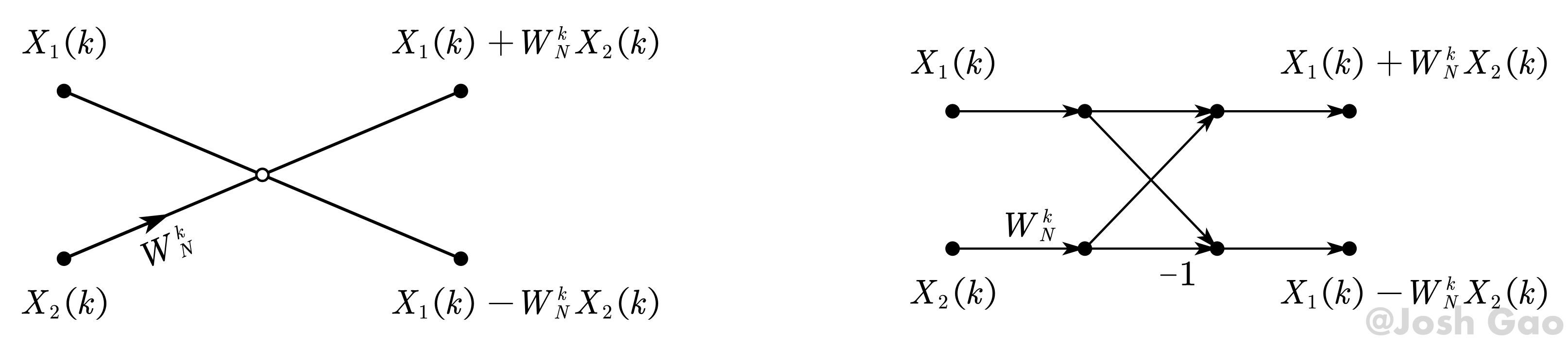+![基-2 按时间抽取的 FFT 算法的鲽形图](https://josh-blog-1257563604.cos.ap-beijing.myqcloud.com/img/2023-04-14-josh-dsp-part-4/2023-04-14-josh-dsp-part-4-010-Radix2DITFFTButterfly.png?imageMogr2/thumbnail/!100p|watermark/2/text/QEpvc2ggR2Fv/font/YWhyb25iZC50dGY=/fontsize/80/dissolve/20/gravity/southeast/dx/5/dy/5){width=1000px}
+
+## 3.3 8 点基-2 DIT-FFT 推导
+
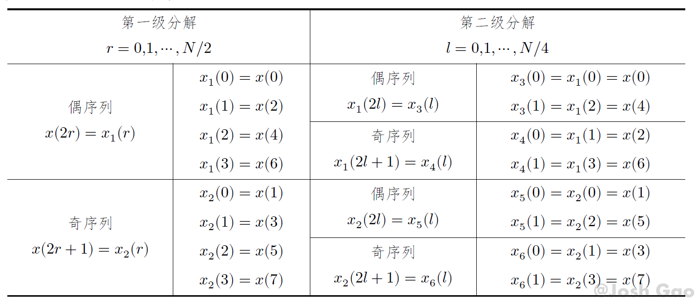+![8 点 radix-2 DIT-FFT 推导](https://josh-blog-1257563604.cos.ap-beijing.myqcloud.com/img/2023-04-14-josh-dsp-part-4/2023-04-14-josh-dsp-part-4-020-Radix2DITFFTDerivation.png?imageMogr2/thumbnail/!100p|watermark/2/text/QEpvc2ggR2Fv/font/YWhyb25iZC50dGY=/fontsize/40/dissolve/20/gravity/southeast/dx/5/dy/5){width=1000px}
+
+&emsp;&emsp;对于 8 点的序列，进行两次分解后每部分序列只含有两个点，可以直接计算 DFT。为了得到自然顺序输出的 DFT 序列，将第二级分解以后的结果作为输入。下面推导每级分解后序列的结果表示。
+
+&emsp;&emsp;对于第一级分解，直接用[算法原理](#3.1)中的式子表示结果，有
+
+$$\begin{align}
+&X\left(k\right)=X_1\left(k\right)+W_N^kX_2\left(k\right),&k=0,1,\cdots,\frac{N}{2}\\
+&X\left(k+\frac{N}{2}\right)=X_1\left(k\right)+W_N^kX_2\left(k\right),&k=0,1,\cdots,\frac{N}{2}
+\end{align}$$
+
+对于第二级分解
+
+$$\begin{equation}
+\begin{aligned}
+X_1\left(k\right)&=\sum_{l=0}^{\frac{N}{4}-1}{x_1\left(2l\right)W_{\frac{N}{2}}^{2lk}}+\sum_{l=0}^{\frac{N}{4}-1}{x_1\left(2l+1\right)W_{\frac{N}{2}}^{\left(2l+1\right)k}}
+\\
+&=\sum_{l=0}^{\frac{N}{4}-1}{x_3\left(l\right)W_{\frac{N}{4}}^{lk}}+W_{\frac{N}{2}}^k\sum_{l=0}^{\frac{N}{4}-1}{x_4\left(l\right)W_{\frac{N}{4}}^{lk}}=X_3\left(k\right)+W_{\frac{N}{2}}^kX_4\left(k\right),\ \ k=0,1,\cdots,\frac{N}{4}-1
+\end{aligned}
+\end{equation}$$
+
+$$\begin{equation}
+X_1\left(k+\frac{N}{4}\right)=X_3\left(k\right)-W_{\frac{N}{2}}^kX_4\left(k\right),\ \ k=0,1,\cdots,\frac{N}{4}-1
+\end{equation}$$
+
+同理
+
+$$\begin{equation}
+X_2\left(k\right)=X_5\left(k\right)+W_{\frac{N}{2}}^kX_6\left(k\right),X_2\left(k+\frac{N}{2}\right)=X_5\left(k\right)-W_{\frac{N}{2}}^kX_6\left(k\right),\ \ k=0,1,\cdots,\frac{N}{4}-1
+\end{equation}$$
+
+对于最后剩下的四个 $\dfrac{N}{4}=2$ 点的 DFT，即 $X_3\left(k\right)、X_4\left(k\right)、X_5\left(k\right)、X_6\left(k\right)，k=0,1$，可按定义计算，如对 $X_3\left(k\right)$
+
+$$\begin{equation}
+\begin{aligned}
+&X_3\left(k\right)=\sum_{l=0}^{\frac{N}{4}-1}{x_3\left(l\right)W_{\frac{N}{4}}^{lk}}=\sum_{l=0}^{1}{x_3\left(l\right)W_{\frac{N}{4}}^{lk}}\\
+\Longrightarrow &X_3\left(0\right)=x_3\left(0\right)+W_2^0x_3\left(1\right)=x\left(0\right)+W_N^0x\left(4\right),X_3\left(1\right)=x_3\left(0\right)+W_2^1x_3\left(1\right)=x\left(0\right)-W_N^0x\left(4\right)
+\end{aligned}
+\end{equation}$$
+
+将上述各式的旋转因子统一为 $W_{\frac{N}{2}}^k=W_N^{2k}$，则一个 8 点的 DFT 可以分解为四个 $\dfrac{N}{4}$ 点的 DFT ，先做 $\dfrac{N}{4}$ 点的 DFT，再用相应的两个 $\dfrac{N}{4}$ 点 DFT 的结果合成 $\dfrac{N}{2}$ 点的 DFT，从而得到 $X_1\left(k\right)、X_2\left(k\right)$，最后组合成为 $N$ 点的 DFT。上述过程的运算流图如下左图，实际绘制按照如下右图即可。
+
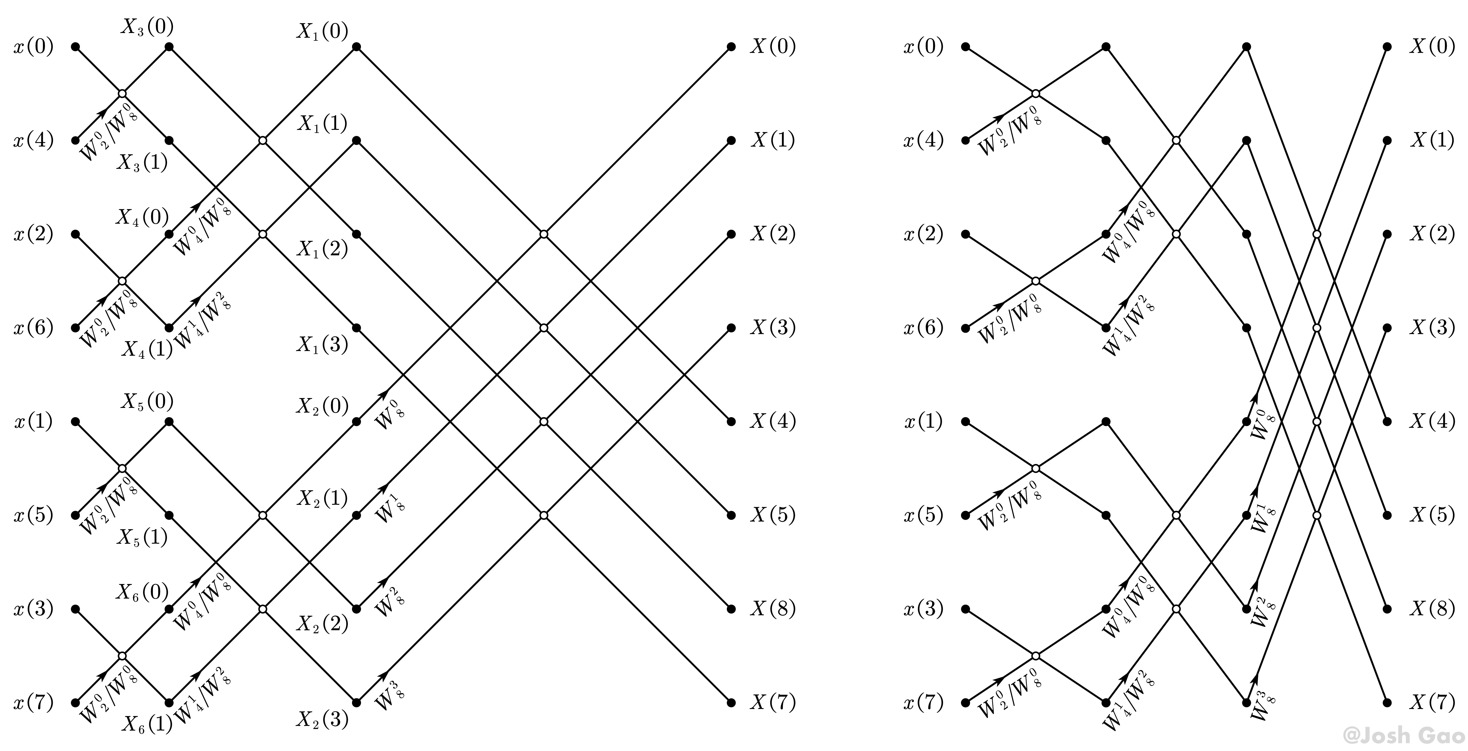+![8 点 radix-2 DIT-FFT 的蝶形图](https://josh-blog-1257563604.cos.ap-beijing.myqcloud.com/img/2023-04-14-josh-dsp-part-4/2023-04-14-josh-dsp-part-4-030-8PointRadix2DITFFTButterfly.png?imageMogr2/thumbnail/!100p|watermark/2/text/QEpvc2ggR2Fv/font/YWhyb25iZC50dGY=/fontsize/80/dissolve/20/gravity/southeast/dx/5/dy/5){width=1000px}
+
+## 3.4 算法特点
+
+### 3.4.1 原位运算
+
+&emsp;&emsp;每级计算所得点数相同，且上一级数据不影响下级运算，数据可以保存在原寄存器中。
+
+### 3.4.2 比特反位序
+
+&emsp;&emsp;若下标 $n$ 可用二进制表示为 $n=\left(b_2b_1b_0\right)_2$，则 FFT 的输入样本序号 $k$ 就可用二进制表示为 $k=\left(b_0b_1b_2\right)_2$。
+
+### 3.4.3 计算复杂度
+
+&emsp;&emsp;对于长度为 $N=2^\nu$ 的序列，共有 $\nu$ 级蝶形运算，每级有 $\dfrac{N}{2}$ 个蝶形，每个蝶形有 $1$ 次复数加法、$2$ 次复数乘法，因此 $\nu$ 级蝶形运算共有
+
+$$\begin{equation}
+\begin{aligned}
+&复数乘法：m_F=\frac{N}{2}\cdot\nu=\frac{N}{2}\log_2{N}\\
+&复数加法：a_F=N\cdot\nu=N\log_2{N}
+\end{aligned}
+\end{equation}$$
+
+### 3.4.4 各类蝶形运算两个点相距的“距离”及 $W_N^k$ 的变化规律
+
+| 点数 $N$ | 列数 | 蝶形运算的种类数 | 蝶形运算的系数 | 参加蝶形运算的<br>两数据点的间距
+| :--: | :--: | :--: | :--: | :--: |
+| $\top$ | 第 $1$ 列 | $1$ 种 | $W_2^0/W_8^0=1$ | $1$ |
+| $8$ | 第 $2$ 列 | $2$ 种 | $W_4^0/W_8^0,{W_4^1/W}_8^2$ | $2$ |
+| $\bot$ | 第 $3$ 列 | $4$ 种 | $W_8^0,W_8^1,W_8^2,W_8^3$ | $4$ |
+| $\top$ | 第 $1$ 列 | $2^0$ 种 | $W_2^0/W_N^0$ | $1$ |
+| $\mid$ | 第 $2$ 列 | $2^1$ 种 | $W_4^0/W_N^0,{W_4^1/W}_N^{\frac{N}{4}}$ | $2$ |
+| $\mid$ | 第 $3$ 列 | $2^2$ 种 | $W_8^0,W_8^1,W_8^2,W_8^3/$<br>$W_N^0,W_N^{\frac{8}{N}},W_N^{2\cdot\frac{8}{N}},W_8^{3\cdot\frac{8}{N}}$ | $4$ |
+| $2^\nu$ | $\vdots$ | $\vdots$ | $\vdots$ | $\vdots$ |
+| $\mid$ | 第 $\nu-1$ 列 | $2^{\nu-2}$ 种 | $W_{\frac{N}{2}}^0,W_{\frac{N}{2}}^1,W_{\frac{N}{2}}^2,\cdots,W_{\frac{N}{2}}^{\frac{N}{4}-1}$ $W_N^0,W_N^2,W_N^4,\cdots,W_N^{\frac{N}{2}-2}$ | $\dfrac{N}{4}$ |
+| $\bot$ | 第 $\nu$ 列 | $2^{\nu-1}$ 种 | $W_N^0,W_N^1,W_N^2,\cdots,W_N^{\frac{N}{2}-1}$ | $\dfrac{N}{2}$ |
+
+&emsp;&emsp;以上述 8 点 FFT 为例，各列蝶形运算的种类数和系数以及参加蝶形运算的两数据点的间距如上表上半部。可见，每列的蝶形类型比前一列增加一倍，参加蝶形运算的两个数据点的间距也增大一倍。最后一列系数用的最多，为 4 个，即 $W_8^0,W_8^1,W_8^2,W_8^3$；而前一列只用带它偶序号的那一半，即 ${W_4^0/W}_8^0,{W_4^1/W}_8^2$；第一列只有一个系数即 ${W_2^0/W}_8^0$。
+
+&emsp;&emsp;上述结论可推广至 $N=2^\nu$ 的一般情况。如上表下半部。从前向后，第一列只有一种类型的蝶形运算 $W_N^0$，以后的每列蝶形的类型逗逼前一列增加一倍，到第 $\nu$ 列是 $\dfrac{N}{2}$ 个蝶形类型，系数是 $W_N^0,W_N^1,\cdots,W_N^{\frac{N}{2}-1}$，共 $\dfrac{N}{2}$ 个。从后向前，系数是后一级的偶数序号的那一半。参加蝶形运算的两个数据点的间距，是最末一级最大，其值为 $\dfrac{N}{2}$，向前每推进一列，间距减少一半。
+
+# 4. 基-2 按频率抽取的 FFT 算法
+
+（radix-2 Decimation in Frequency Fast Fourier Transform, radix-2 DIF-FFT, i.e. Sande-Tukey Method）
+
+## 4.1 算法原理
+
+&emsp;&emsp;设序列 $x\left(n\right)的列长N=2^\nu$，$\nu$ 为整数，则其 DFT
+
+$$\begin{equation}
+X\left(k\right)=\sum_{n=0}^{N-1}{x\left(n\right)W_N^{nk}},\ \ k=0,1,\cdots,N-1
+\end{equation}$$
+
+**将 $x\left(n\right)$ 按照 $n$ 的顺序分成两个子序列（即可将 $X\left(k\right)$ 按照奇偶分组）**
+
+$$\begin{equation}
+\begin{cases}
+前半子序列x\left(n\right)\\
+后半子序列x\left(n+\dfrac{N}{2}\right)
+\end{cases}
+,\ \ n=0,1,\cdots,\frac{N}{2}-1
+\end{equation}$$
+
+则序列的 DFT 可表示为
+
+$$\begin{equation}
+\begin{aligned}
+X\left(k\right)&=\sum_{n=0}^{\frac{N}{2}-1}{x\left(n\right)W_N^{nk}}+\sum_{n=\frac{N}{2}}^{N-1}{x\left(n\right)W_N^{nk}}=\sum_{n=0}^{\frac{N}{2}-1}{x\left(n\right)W_N^{nk}}+\sum_{n=0}^{\frac{N}{2}-1}{x\left(n+\frac{N}{2}\right)W_N^{(n+\frac{N}{2})k}}
+\\
+&=\sum_{n=0}^{\frac{N}{2}-1}{\left[x\left(n\right)+W_N^{\frac{N}{2}k}x\left(n+\frac{N}{2}\right)\right]W_N^{nk}}
+\\
+&\xlongequal{W_{N}^{\frac{N}{2}k}=\left( -1 \right) ^k}\sum_{n=0}^{\frac{N}{2}-1}{\left[x\left(n\right)+\left(-1\right)^kx\left(n+\frac{N}{2}\right)\right]W_N^{nk}},\ \ k=0,1,\cdots,\frac{N}{2}-1
+\end{aligned}
+\end{equation}$$
+
+由 $W_N^{\frac{N}{2}k}=\left(-1\right)^k$，按照 $k$ 的奇偶可将 $X\left(k\right)$ 分成两部分，令 $k=2r$ 及 $k=2r+1,\ r=0,1,\cdots,\dfrac{N}{2}-1$，则
+
+$$\begin{align}
+&X\left(2r\right)=\sum_{n=0}^{\frac{N}{2}-1}{\left[x\left(n\right)+x\left(n+\frac{N}{2}\right)\right]W_N^{2rn}}=\sum_{n=0}^{\frac{N}{2}-1}{\left[x\left(n\right)+x\left(n+\frac{N}{2}\right)\right]W_{\frac{N}{2}}^{rn}}
+\\
+&X\left(2r+1\right)=\sum_{n=0}^{\frac{N}{2}-1}{\left[x\left(n\right)-x\left(n+\frac{N}{2}\right)\right]W_N^{2rn}}=\sum_{n=0}^{\frac{N}{2}-1}{\left[x\left(n\right)-x\left(n+\frac{N}{2}\right)\right]W_N^nW_{\frac{N}{2}}^{rn}}
+\end{align}$$
+
+上两式种的前者是输入序列前一半和后一半之和的 $\dfrac{N}{2}$ 点 DFT，后者是输入序列前一半和后一半之差与 $W_N^n$ 之积的 $\dfrac{N}{2}$ 点 DFT。令
+
+$$\begin{equation}
+\begin{cases}
+x_1\left(n\right)=x\left(n\right)+x\left(n+\dfrac{N}{2}\right)\\
+x_2\left(n\right)=\left[x\left(n\right)-x\left(n+\dfrac{N}{2}\right)\right]W_N^n
+\end{cases}
+,\ \ n=0,1,\cdots,\frac{N}{2}-1
+\end{equation}$$
+
+则
+
+$$\begin{equation}
+X\left(2r\right)=\sum_{n=0}^{\frac{N}{2}-1}{x_1\left(n\right)W_{\frac{N}{2}}^{rn}},\ \ X\left(2r+1\right)=\sum_{n=0}^{\frac{N}{2}-1}{x_2\left(n\right)W_{\frac{N}{2}}^{rn}}
+\end{equation}$$
+
+由此，可将 $N$ 点 DFT 按频率 $k$ 的奇偶分解为两个序列的 $\dfrac{N}{2}$ 点 DFT。类似地，可以将分离后的序列继续按频率k的奇偶分成两个序列计算，**直到每个序列中只含有两个点**。此时开始计算 DFT。这种方法称为**基-2 按频率抽取的 FFT 算法**。
+
+## 4.2 蝶形运算流图符号
+
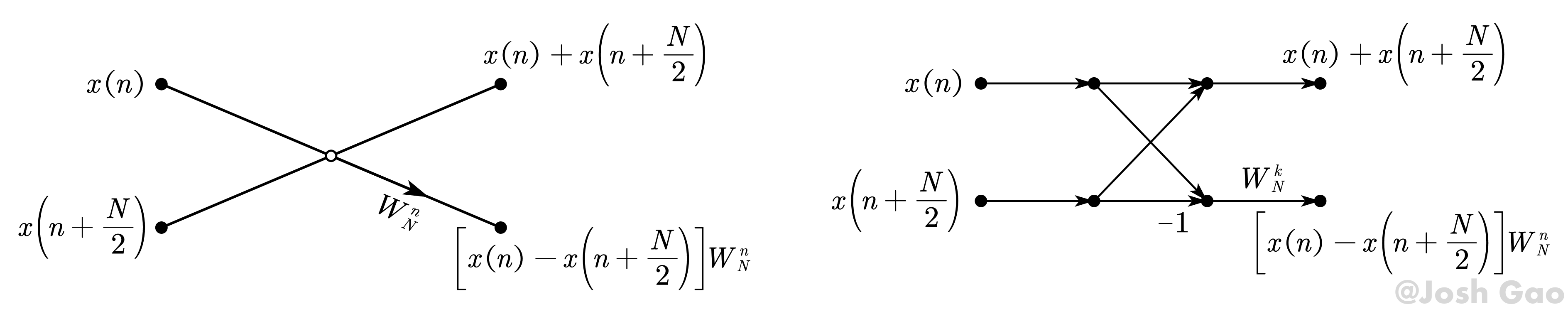+![基-2 按频率抽取的 FFT 算法的蝶形图](https://josh-blog-1257563604.cos.ap-beijing.myqcloud.com/img/2023-04-14-josh-dsp-part-4/2023-04-14-josh-dsp-part-4-040-Radix2DIFFFTButterfly.png?imageMogr2/thumbnail/!100p|watermark/2/text/QEpvc2ggR2Fv/font/YWhyb25iZC50dGY=/fontsize/80/dissolve/20/gravity/southeast/dx/5/dy/5){width=1000px}
+
+## 4.3 8 点基-2 DIF-FFT 推导简述
+
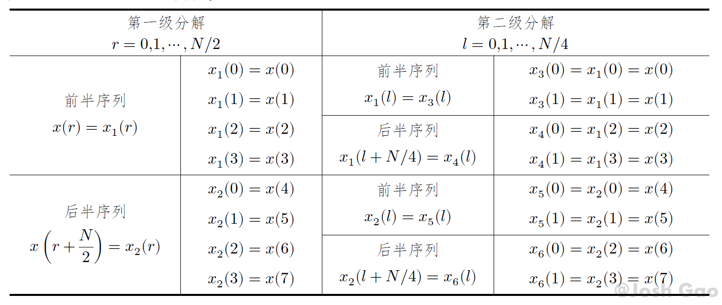+![8 点 radix-2 DIF-FFT 推导](https://josh-blog-1257563604.cos.ap-beijing.myqcloud.com/img/2023-04-14-josh-dsp-part-4/2023-04-14-josh-dsp-part-4-050-Radix2DIFFFTDerivation.png?imageMogr2/thumbnail/!100p|watermark/2/text/QEpvc2ggR2Fv/font/YWhyb25iZC50dGY=/fontsize/40/dissolve/20/gravity/southeast/dx/5/dy/5){width=1000px}
+
+运算流图如下左图，实际绘制按照如下右图即可。
+
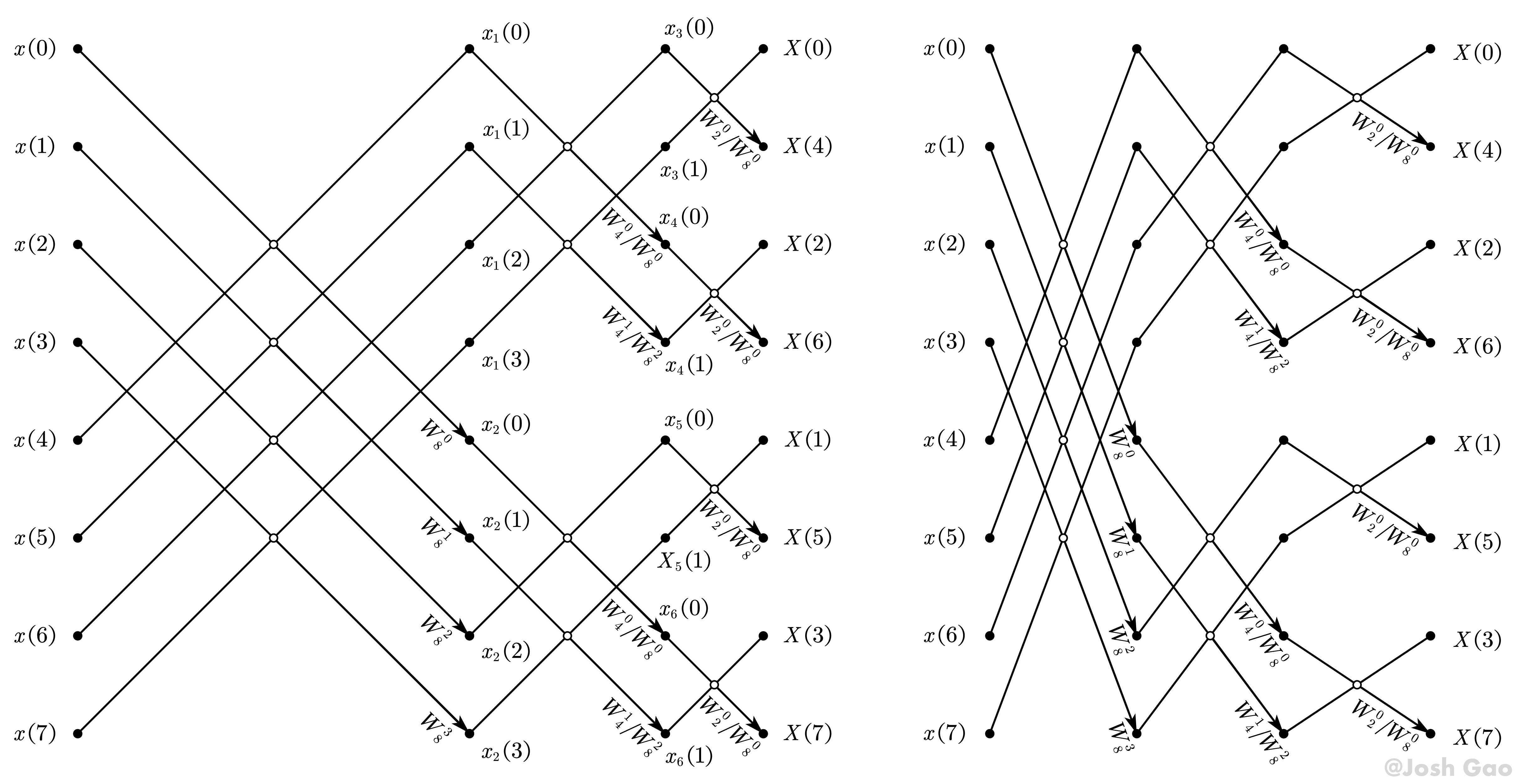+![8 点 radix-2 DIF-FFT 的蝶形图](https://josh-blog-1257563604.cos.ap-beijing.myqcloud.com/img/2023-04-14-josh-dsp-part-4/2023-04-14-josh-dsp-part-4-060-8PointRadix2DIFFFTButterfly.png?imageMogr2/thumbnail/!100p|watermark/2/text/QEpvc2ggR2Fv/font/YWhyb25iZC50dGY=/fontsize/80/dissolve/20/gravity/southeast/dx/5/dy/5){width=1000px}
+
+**对于任何流图，只要保持各节点所连的支路及其传输系数不变，则不论节点位置怎么排列，所得流图总是等效的，最后所得 DFT 结果也是正确的**，只是数据的提取和存放次序不同而已。
+
+## 4.4 算法特点
+
+### 4.4.1 原位运算
+
+&emsp;&emsp;每级计算所得点数相同，且上一级数据不影响下级运算，数据可以保存在原寄存器中。
+
+### 4.4.2 比特反位序
+
+&emsp;&emsp;若下标 $n$ 可用二进制表示为 $n=\left(b_2b_1b_0\right)_2$，则 FFT 的输入样本序号 $k$ 就可用二进制表示为 $k=\left(b_0b_1b_2\right)_2$。
+
+### 4.4.3 计算复杂度
+
+&emsp;&emsp;对于长度为 $N=2^\nu$ 的序列，共有 $\nu$ 级蝶形运算，每级有 $\dfrac{N}{2}$ 个蝶形，每个蝶形有 $1$ 次复数加法、$2$ 次复数乘法，因此 $\nu$ 级蝶形运算共有
+
+$$\begin{equation}
+\begin{aligned}
+&复数乘法：m_F=\frac{N}{2}\cdot\nu=\frac{N}{2}\log_2{N}\\
+&复数加法：a_F=N\cdot\nu=N\log_2{N}
+\end{aligned}
+\end{equation}$$
+
+# 5. 基-2 DIT-FFT 和 基-2 DIF-FFT 的比较
+
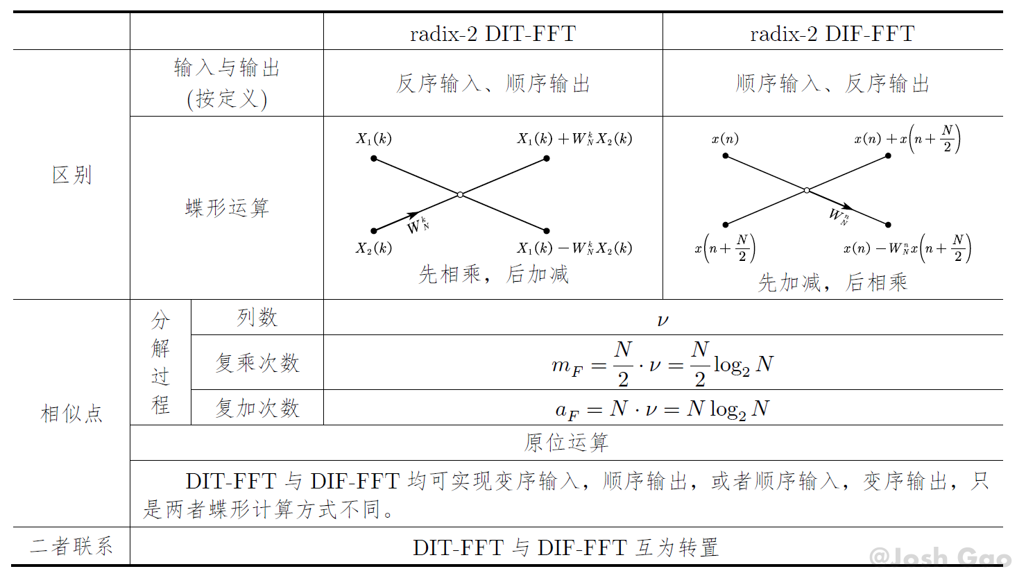+![radix-2 DIT-FFT 和 radix-2 DIF-FFT 的比较](https://josh-blog-1257563604.cos.ap-beijing.myqcloud.com/img/2023-04-14-josh-dsp-part-4/2023-04-14-josh-dsp-part-4-070-Radix2DIFFFTRadix2DIFFFTComparison.png?imageMogr2/thumbnail/!100p|watermark/2/text/QEpvc2ggR2Fv/font/YWhyb25iZC50dGY=/fontsize/40/dissolve/20/gravity/southeast/dx/5/dy/5){width=1000px}
+
+# 6. 分裂基 FFT 算法（split-radix FFT Method）
+
+## 6.1 算法原理（基-4 DIF-FFT同理）
+
+&emsp;&emsp;设序列 $x\left(n\right)$ 的列长 $N=2^\nu$，$\nu$为整数，则其 DFT
+
+$$\begin{equation}
+X\left(k\right)=\sum_{n=0}^{N-1}{x\left(n\right)W_N^{nk}},\ \ k=0,1,\cdots,N-1
+\end{equation}$$
+
+将 $x\left(n\right)$ 按照 $n$ 的顺序分成四个子序列
+
+$$\begin{equation}
+\begin{cases}
+第一子序列x\left(n\right)\\
+第二子序列x\left(n+\dfrac{N}{4}\right)\\
+第三子序列x\left(n+\dfrac{N}{2}\right)\\
+第四子序列x\left(n+\dfrac{3N}{4}\right)
+\end{cases}
+,\ \ n=0,1,\cdots,\frac{N}{2}-1
+\end{equation}$$
+
+则序列的 DFT 可表示为
+
+$$\begin{equation}
+\begin{aligned}
+X\left(k\right)&=\sum_{n=0}^{\frac{N}{4}-1}{x\left(n\right)W_N^{nk}}+\sum_{n=\frac{N}{4}}^{\frac{N}{2}-1}{x\left(n\right)W_N^{nk}}+\sum_{n=\frac{N}{2}}^{\frac{3N}{4}-1}{x\left(n\right)W_N^{nk}}+\sum_{n=\frac{3N}{4}}^{N-1}{x\left(n\right)W_N^{nk}}
+\\
+&=\sum_{n=0}^{\frac{N}{4}-1}\left[x\left(n\right)W_N^{nk}+x\left(n+\frac{N}{4}\right)W_N^{\left(n+\frac{N}{4}\right)k}+x\left(n+\frac{N}{2}\right)W_N^{\left(n+\frac{N}{2}\right)k}+x\left(n+\frac{3N}{4}\right)W_N^{\left(n+\frac{3N}{4}\right)k}\right]
+\\
+&=\sum_{n=0}^{\frac{N}{4}-1}{\left[x\left(n\right)+x\left(n+\frac{N}{4}\right)W_N^{\frac{N}{4}k}+x\left(n+\frac{N}{2}\right)W_N^{\frac{N}{2}k}+x\left(n+\frac{3N}{4}\right)W_N^{\frac{3N}{4}k}\right]W_N^{nk}}
+\\
+&=\sum_{n=0}^{\frac{N}{4}-1}{\left[x\left(n\right)+x\left(n+\frac{N}{4}\right)W_4^k+x\left(n+\frac{N}{2}\right)W_4^{2k}+x\left(n+\frac{3N}{4}\right)W_4^{3k}\right]W_N^{nk}}
+\end{aligned}
+\end{equation}$$
+
+按照 $k$ 除以 $4$ 的余数可将 $X\left(k\right)$ 分成四部分，分别令 $k=4r、k=4r+1、k=4r+2、k=4r+3$，其中 $r=0,1,\cdots,\dfrac{N}{4}-1$，则有
+
+$$\begin{equation}
+\begin{cases}
+X\left(4r\right)=\displaystyle\sum_{n=0}^{\frac{N}{4}-1}{\left[x\left(n\right)+x\left(n+\dfrac{N}{4}\right)+x\left(n+\dfrac{N}{2}\right)+x\left(n+\dfrac{3N}{4}\right)\right]W_{\frac{N}{4}}^{rn}}
+\\
+X\left(4r+1\right)=\displaystyle\sum_{n=0}^{\frac{N}{4}-1}{\left[x\left(n\right)-jx\left(n+\dfrac{N}{4}\right)-x\left(n+\dfrac{N}{2}\right)+jx\left(n+\dfrac{3N}{4}\right)\right]W_N^nW_{\frac{N}{4}}^{rn}}
+\\
+X\left(4r+2\right)=\displaystyle\sum_{n=0}^{\frac{N}{4}-1}{\left[x\left(n\right)-x\left(n+\dfrac{N}{4}\right)+x\left(n+\dfrac{N}{2}\right)-x\left(n+\dfrac{3N}{4}\right)\right]W_N^{2n}W_{\frac{N}{4}}^{rn}}
+\\
+X\left(4r+3\right)=\displaystyle\sum_{n=0}^{\frac{N}{4}-1}{\left[x\left(n\right)+jx\left(n+\dfrac{N}{4}\right)-x\left(n+\dfrac{N}{2}\right)-jx\left(n+\dfrac{3N}{4}\right)\right]W_N^{3n}W_{\frac{N}{4}}^{rn}}
+\end{cases}
+,\ \ r=0,1,\cdots,\frac{N}{4}-1
+\end{equation}$$
+
+上述过程也是基-4 DIF-FFT 的推导。上式中的偶数序号项合并，得
+
+$$\begin{equation}
+\begin{cases}
+X\left(2r\right)=\displaystyle\sum_{n=0}^{\frac{N}{2}-1}{\left[x\left(n\right)+x\left(n+\dfrac{N}{2}\right)\right]W_N^{2rn}}, &r=0,1,\cdots,\dfrac{N}{2}-1
+\\
+X\left(4r+1\right)=\displaystyle\sum_{n=0}^{\frac{N}{4}-1}{\left[\left(x\left(n\right)-x\left(n+\dfrac{N}{2}\right)\right)-j\left(x\left(n+\dfrac{N}{4}\right)-x\left(n+\dfrac{3N}{4}\right)\right)\right]W_N^nW_{\frac{N}{4}}^{rn}},&r=0,1,\cdots,\dfrac{N}{4}-1
+\\
+X\left(4r+3\right)=\displaystyle\sum_{n=0}^{\frac{N}{4}-1}{\left[\left(x\left(n\right)-x\left(n+\dfrac{N}{2}\right)\right)+j\left(x\left(n+\dfrac{N}{4}\right)-x\left(n+\dfrac{3N}{4}\right)\right)\right]W_N^{3n}W_{\frac{N}{4}}^{rn}},&r=0,1,\cdots,\dfrac{N}{4}-1
+\end{cases}
+\end{equation}$$
+
+令
+
+$$\begin{equation}
+\begin{cases}
+x_2\left(n\right)=x\left(n\right)+x\left(n+\dfrac{N}{2}\right), &n=0,1,\cdots,\dfrac{N}{2}-1
+\\
+x_4^1\left(n\right)=\left[\left(x\left(n\right)-x\left(n+\dfrac{N}{2}\right)\right)-j\left(x\left(n+\dfrac{N}{4}\right)-x\left(n+\dfrac{3N}{4}\right)\right)\right]W_N^n,&n=0,1,\cdots,\dfrac{N}{4}-1
+\\
+x_4^2\left(n\right)=\left[\left(x\left(n\right)-x\left(n+\dfrac{N}{2}\right)\right)+j\left(x\left(n+\dfrac{N}{4}\right)-x\left(n+\dfrac{3N}{4}\right)\right)\right]W_N^{3n},&n=0,1,\cdots,\dfrac{N}{4}-1
+\end{cases}
+\end{equation}$$
+
+则有
+
+$$\begin{equation}
+\begin{cases}
+X\left(2r\right)=\displaystyle\sum_{n=0}^{\frac{N}{2}-1}{x_2\left(n\right)W_{\frac{N}{2}}^{rn}}=DFT\left[x_2\left(n\right)\right], &r=0,1,\cdots,\dfrac{N}{2}-1
+\\
+X\left(4r+1\right)=\displaystyle\sum_{n=0}^{\frac{N}{4}-1}{x_4^1\left(n\right)W_{\frac{N}{4}}^{rn}}=\mathrm{DFT}\left[x_4^1\left(n\right)\right],&r=0,1,\cdots,\dfrac{N}{4}-1
+\\
+X\left(4r+3\right)=\displaystyle\sum_{n=0}^{\frac{N}{4}-1}{x_4^2\left(n\right)W_{\frac{N}{4}}^{rn}}=\mathrm{DFT}\left[x_4^2\left(n\right)\right],&r=0,1,\cdots,\dfrac{N}{4}-1
+\end{cases}
+\end{equation}$$
+
+由此，DFT 的偶数部分采用基-2 算法，奇数部分采用基-4 算法，将一个 $N$ 点 DFT 的分解为一个 $\dfrac{N}{2}$ 点 DFT 和两个 $\dfrac{N}{4}$ 点 DFT。可将分裂基-2/4 算法看成**时域分段、频域抽取**的方法。先将整个 $N$ 点序列在时域分成两段，对于偶数段，在时域进一步分成两段，相当于在频域抽取偶数点 $X\left(2r\right)$；对于奇数段，在时域分成 4 段，相当于在频域抽取奇数点 $X\left(4r+1\right)$ 和 $X\left(4r+3\right)$。类似地，可将分离后的序列继续分解，直到最后一级。这种方法称为**分裂基 FFT 算法**。
+
+## 6.2 L 蝶形运算流图符号
+
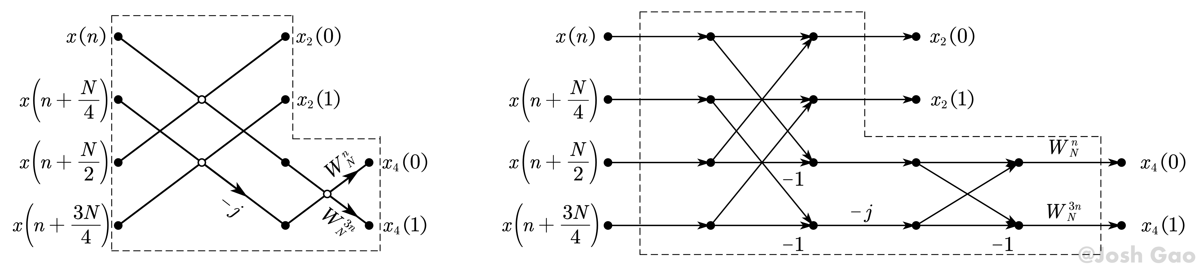+![L 蝶形运算流图符号](https://josh-blog-1257563604.cos.ap-beijing.myqcloud.com/img/2023-04-14-josh-dsp-part-4/2023-04-14-josh-dsp-part-4-080-Radix24LButterfly.png?imageMogr2/thumbnail/!100p|watermark/2/text/QEpvc2ggR2Fv/font/YWhyb25iZC50dGY=/fontsize/80/dissolve/20/gravity/southeast/dx/5/dy/5){width=1000px}
+
+## 6.3 8 点 radix-2/4 FFT举例
+
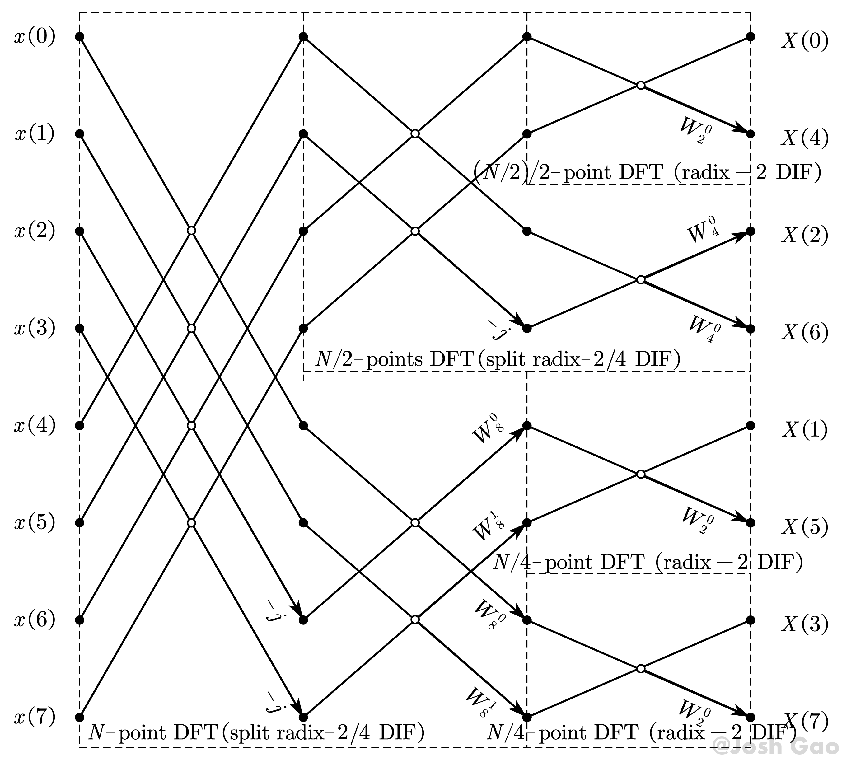+![8 点 radix-2/4 FFT举例](https://josh-blog-1257563604.cos.ap-beijing.myqcloud.com/img/2023-04-14-josh-dsp-part-4/2023-04-14-josh-dsp-part-4-090-8PointRadix24LButterfly.png?imageMogr2/thumbnail/!100p|watermark/2/text/QEpvc2ggR2Fv/font/YWhyb25iZC50dGY=/fontsize/80/dissolve/20/gravity/southeast/dx/5/dy/5){width=600px}
+
+## 6.4 运算量分析
+
+&emsp;&emsp;对于 $N=2^\nu$ 点 DFT，设第 $i$ 级有 $l_i$ 个蝶形，$j=0,1,\cdots,\nu-1$，则
+
+$$\begin{equation}
+\begin{cases}
+l_1=\dfrac{N}{4}\\
+l_i=\dfrac{N}{4}-\dfrac{l_{j-1}}{2}=\dfrac{N}{6}\left[1-\left(-\dfrac{1}{2}\right)^i\right],\ \ i\neq1
+\end{cases}
+\Longrightarrow\sum_{i=1}^{\nu-1}l_i=\frac{N}{6}\left[\nu-\frac{2}{3}+\frac{2}{3}\left(-\frac{1}{2}\right)^\nu\right]
+\end{equation}$$
+
+其中 $l_i$ 来自 L 蝶形的特殊结构。总的复乘次数为 L 蝶形数的两倍，而总的复加次数与基-2 FFT 算法相同，即
+
+$$\begin{equation}
+\begin{aligned}
+&复数乘法：C_F=2\cdot\sum_{i=1}^{\nu-1}l_i=\frac{N}{3}\log_2{N}-\frac{2N}{9}+\frac{\left(-1\right)^\nu2}{9}\ \ \propto\ \ \frac{N}{3}\log_2{N}\\
+&复数加法：a_F=N\cdot\nu=N\log_2{N}
+\end{aligned}
+\end{equation}$$
+
+显然，**复乘次数相比基-2 FFT 算法下降了33%**。
+
+> **L 蝶形数与流图中 $-j$ 的个数相等。**
+
+# 7. 实序列的 FFT 算法
+
+## 7.1 用一个 $N$ 点 DFT 同时计算两个 $N$ 点实序列的 DFT
+
+&emsp;&emsp;设 $x_1\left(n\right),x_2\left(n\right)$ 是相互独立的两个 $N$ 点实序列，将 $x_1\left(n\right)$ 和 $x_2\left(n\right)$ 分别当作一复序列的实部和虚部，即
+
+$$\begin{equation}
+x\left(n\right)=x_1\left(n\right)+jx_2\left(n\right)
+\end{equation}$$
+
+则由 DFT 的线性性质，$x\left(n\right)$ 的 DFT 可表示为
+
+$$\begin{equation}
+X\left(k\right)=X_1\left(k\right)+jX_2\left(k\right)
+\end{equation}$$
+
+再由的[复序列的 DFT 性质](https://josh-gao.top/posts/fd9f9a29.html#共轭复序列的-dft)
+
+$$\begin{equation}
+X\left(k\right)=X_{ep}\left(k\right)+X_{op}\left(k\right)
+\end{equation}$$
+
+则有 $X_1\left(k\right)$ 和 $X_2\left(k\right)$
+
+$$\begin{equation}
+X_1\left(k\right)=X_{ep}\left(k\right)=\frac{1}{2}\left[X\left(k\right)+X^\ast\left(N-k\right)\right]
+\end{equation}$$
+
+$$\begin{equation}
+X_2\left(k\right)=-{jX}_{op}\left(k\right)=-\frac{j}{2}\left[X\left(k\right)-X^\ast\left(N-k\right)\right]
+\end{equation}$$
+
+蝶形图如下：
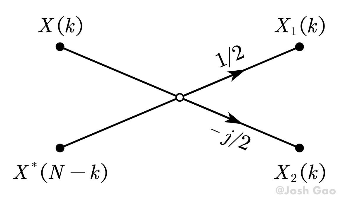+![用一个 N点 DFT 同时计算两个 N 点实序列的 DFT的蝶形图](https://josh-blog-1257563604.cos.ap-beijing.myqcloud.com/img/2023-04-14-josh-dsp-part-4/2023-04-14-josh-dsp-part-4-100-ComputeNPointComplxDFT.png?imageMogr2/thumbnail/!100p|watermark/2/text/QEpvc2ggR2Fv/font/YWhyb25iZC50dGY=/fontsize/40/dissolve/20/gravity/southeast/dx/5/dy/5){width=500px}
+
+## 7.2 用一个 $N$ 点 DFT 计算一个 $2N$ 点实序列的 DFT
+
+&emsp;&emsp;设 $x\left(n\right)$ 是一个 $2N$ 点的实序列，将其按照奇偶分为两个独立的 $N$ 点实序列 $x_1\left(n\right),x_2\left(n\right)$，即
+
+$$\begin{equation}
+\begin{cases}
+x_1\left(n\right)=x\left(2n\right)\\
+x_2\left(n\right)=x\left(2n+1\right)
+\end{cases}
+,\ \ n=0,1,\cdots,N-1
+\end{equation}$$
+
+将 $x_1\left(n\right)$ 和 $x_2\left(n\right)$ 分别当作一复序列的实部和虚部，即
+
+$$\begin{equation}
+y\left(n\right)=x_1\left(n\right)+jx_2\left(n\right)
+\end{equation}$$
+
+则由 DFT 的线性性质，$y\left(n\right)$ 的 DFT 可表示为
+
+$$\begin{equation}
+Y\left(k\right)=X_1\left(k\right)+jX_2\left(k\right)
+\end{equation}$$
+
+则由上述讨论，有 $X_1\left(k\right)$ 和 $X_2\left(k\right)$
+
+$$\begin{equation}
+X_1\left(k\right)=Y_{ep}\left(k\right)=\frac{1}{2}\left[Y\left(k\right)+Y^\ast\left(N-k\right)\right]
+\end{equation}$$
+
+$$\begin{equation}
+X_2\left(k\right)=-{jY}_{op}\left(k\right)=-\frac{j}{2}\left[Y\left(k\right)-Y^\ast\left(N-k\right)\right]
+\end{equation}$$
+
+因此 $x\left(n\right)$ 的傅里叶变换（类似基-2 DIT）
+
+$$\begin{equation}
+\begin{aligned}
+X\left(k\right)&=\sum_{n=0}^{2N-1}{x\left(n\right)W_N^{nk}}=\sum_{n=0}^{N-1}{x\left(2n\right)W_{2N}^{2nk}}+\sum_{n=0}^{N-1}{x\left(2n+1\right)W_{2N}^{\left(2n+1\right)k}}
+\\
+&=\sum_{n=0}^{N-1}{x\left(2n\right)W_{2N}^{2nk}}+W_{2N}^k\sum_{n=0}^{N-1}{x\left(2n+1\right)W_{2N}^{2nk}}
+\\
+&=\sum_{n=0}^{N-1}{x_1\left(n\right)W_N^{nk}}+W_{2N}^k\sum_{n=0}^{N-1}{x_2\left(n\right)W_N^{nk}}
+\\
+&=X_1\left(k\right)+W_{2N}^kX_2\left(k\right),\ \ \ \ \ \ \ \ \ \ \ k=0,1,\cdots,N-1
+\end{aligned}
+\end{equation}$$
+
+$$\begin{equation}
+X\left(k+N\right)=X_1\left(k\right)-W_{2N}^kX_2\left(k\right),\ \ k=0,1,\cdots,N-1\qquad\qquad\quad\
+\end{equation}$$
+
+蝶形图如下：
+
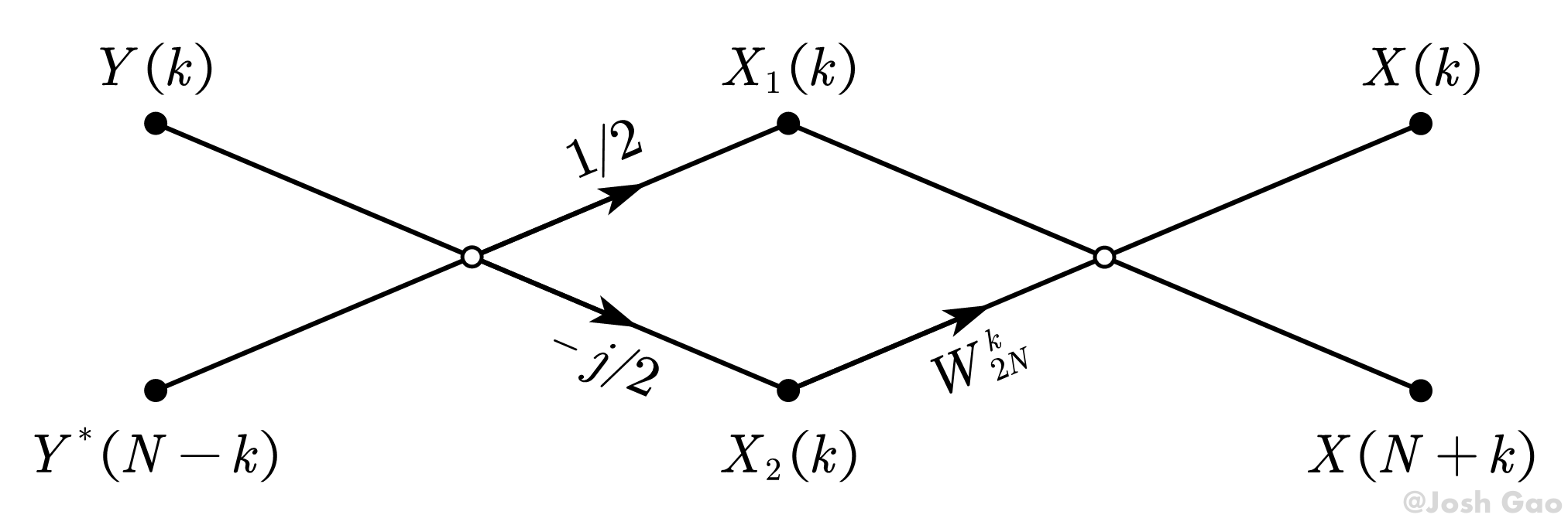+![用一个 N 点 DFT 计算一个 2N 点实序列的 DFT的蝶形图](https://josh-blog-1257563604.cos.ap-beijing.myqcloud.com/img/2023-04-14-josh-dsp-part-4/2023-04-14-josh-dsp-part-4-110-Compute2NPointRealDFT.png?imageMogr2/thumbnail/!100p|watermark/2/text/QEpvc2ggR2Fv/font/YWhyb25iZC50dGY=/fontsize/40/dissolve/20/gravity/southeast/dx/5/dy/5){width=500px}
+
+# 参考文献
+
+王世一. *数字信号处理, 修订版.* 北京理工大学出版社, 1997.

source/about/index.md

@@ -1,6 +1,8 @@
 ---
-title: about
+title: 关于我
 date: 2020-11-25 16:12:56
 type: about
 comments: false
 ---
+
+你好啊！

source/categories/index.md

@@ -1,5 +1,5 @@
 ---
-title: categories
+title: 文章分类
 date: 2020-11-24 21:28:48
 type: categories
 comments: false